LRFD Philosophy, Reliability, and Limit States

Engineering story

Why LRFD replaced ASD

In 1994, AASHTO published the first LRFD Bridge Design Specifications. The switch away from Allowable Stress Design (ASD) was not fashion — it was a response to a generation of research showing that a single global safety factor could not simultaneously calibrate against the very different uncertainties in dead load, live load, wind, seismic events, and material resistance. Bridges designed to the 1996 Standard Specifications and to the first LRFD editions coexist in the Mid-Atlantic today. Understanding both is a load-rating prerequisite.

In Load and Resistance Factor Design (LRFD), bridges are designed for specific limit states that consider various loads and resistances. These limit states include strength, extreme event, service, and fatigue. Each limit state is a design check whose combination of load factors, load combinations, and resistance factors has been statistically calibrated to a target reliability index β. The remainder of this chapter develops each piece.

Chapter objectives

What you will be able to do

Learning objectives

By the end of this chapter you will be able to:

1Distinguish ASD, LFD, and LRFD philosophies.
2Interpret the reliability index β and its role in code calibration.
3Enumerate every AASHTO limit state and state its purpose.
4Look up load factors γ from AASHTO Tables 3.4.1-1 and 3.4.1-2 and apply them.
5Assemble a Strength I demand for a girder combining DC, DW, and LL+IM.
6Select resistance factors φ for reinforced concrete, prestressed concrete, and structural steel.
7Compute the number of design lanes NL, apply multiple-presence factors m, and dynamic load allowance IM.
8Distinguish the design truck, design tandem, design lane load, and fatigue truck within HL-93.

2.1 — Central equation

The LRFD design inequality

AASHTO LRFD §1.3.2

Every AASHTO LRFD check reduces to a single inequality: the sum of factored force effects must not exceed the factored resistance:

(AASHTO 1.3.2.1-1)

Formula
$\sum \eta_{i}\,\gamma_{i}\,Q_{i} \;\le\; \phi \cdot R_{n} \;=\; R_{r}$

$\eta_{i}$: load modifier for load i (ductility · redundancy · importance)
$\gamma_{i}$: load factor for load type i
$Q_{i}$: force effect from load i [kip, kip-ft]
$\phi$: resistance factor
$R_{n}$: nominal resistance [kip, kip-ft]
$R_{r}$: factored resistance = \phi\,R_{n} [kip, kip-ft]

The elegance of LRFD is that both sides of the inequality are calibrated against their real statistical distributions. A live-load moment with a coefficient of variation (COV) of ~18% receives a heavier factor (γ_LL = 1.75 in Strength I) than a dead-load moment with a COV of ~9% (γ_DC = 1.25). Resistance factors φ reflect the manufacturing scatter of the material and the reliability of the resistance model.

2.2 — Load modifier η

Ductility, redundancy, importance

AASHTO LRFD §1.3.3 – §1.3.5

The load modifier η captures three qualitative attributes of the member being designed. For loads for which a maximum value of γ_i is appropriate:

(AASHTO 1.3.2.1-2)

Formula
$\eta_{i} \;=\; \eta_{D} \cdot \eta_{R} \cdot \eta_{I} \;\ge\; 0.95$

$\eta_{D}$: ductility factor (0.95 – 1.05)
$\eta_{R}$: redundancy factor (0.95 – 1.05)
$\eta_{I}$: operational importance factor (0.95 – 1.05)

For loads for which a minimum value of γ_i is appropriate (uplift, overturning):

(AASHTO 1.3.2.1-3)

Formula
$\eta_{i} \;=\; \frac{1}{\eta_{D} \cdot \eta_{R} \cdot \eta_{I}} \;\le\; 1.0$

Engineering note

For a conventional, redundant, ductile Maryland highway bridge of typical importance,η_D = η_R = η_I = 1.00 → η = 1.00. Nonredundant fracture-critical members drive η_R upward, and MDOT SHA identifies routes carrying emergency traffic as elevated-importance.

2.3 — Limit states

Strength, service, fatigue, extreme event

AASHTO LRFD §1.3.2, §3.4.1

Infographic summarizing AASHTO LRFD limit states — Figure 2.1AASHTO LRFD limit-state hierarchy. Strength states size members against collapse; Service states control cracking, deflection, and slip; Fatigue states address repeated live load; Extreme Event states cover earthquake, ice, and collision.

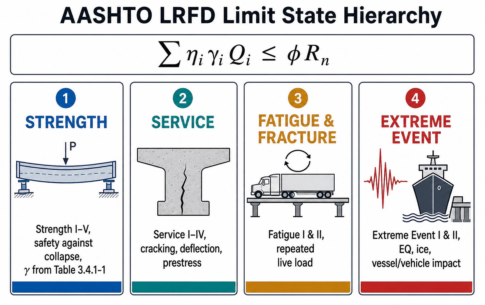
The following limit-state combinations are defined in AASHTO LRFD Article 3.4.1:

Limit state	Purpose
Strength I	Basic vehicular use, no wind. Governs most girder design.
Strength II	Owner-specified special / permit vehicles, no wind.
Strength III	Wind velocity > 55 mph, no live load (empty-bridge wind).
Strength IV	Very high dead/live ratio (spans > ~250 ft).
Strength V	Normal vehicular use with 55 mph wind.
Extreme Event I	Load combination including earthquake.
Extreme Event II	Ice load, vessel or vehicle collision, check flood.
Service I	Normal operational use; deflection check.
Service II	Control yielding of steel and slip of slip-critical connections.
Service III	Tension in prestressed concrete — crack control.
Service IV	Tension in prestressed concrete columns under wind.
Fatigue I	Infinite fatigue life (LL+IM only, γ = 1.5).
Fatigue II	Finite fatigue life (LL+IM only, γ = 0.75).

Table 2.1 — AASHTO limit states (LRFD 10th Ed., §3.4.1). Each combination pairs a defined set of load factors with a target reliability index.

2.4 — Load factors

AASHTO Table 3.4.1-1 (abridged)

AASHTO LRFD §3.4.1

Bar charts of AASHTO LRFD load factors for Strength I and resistance factors phi for common materials — Figure 2.2Left — Strength I load factors: γDC = 1.25, γDW = 1.50, γLL+IM = 1.75, γWA = 1.00. Right — resistance factors φ commonly encountered in Mid-Atlantic design.

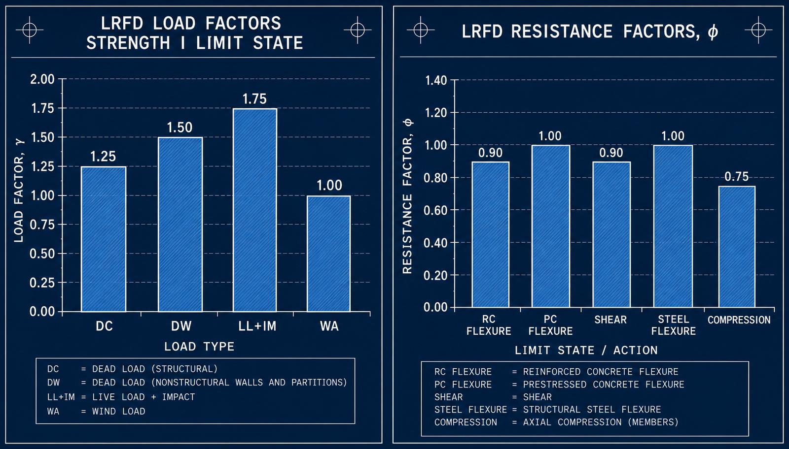
Combination	DC/DW/EH/EV/ES	LL+IM+CE+BR	WA	WS	WL	EQ	CT/CV/IC
Strength I	γp	1.75	1.00	—	—	—	—
Strength II	γp	1.35	1.00	—	—	—	—
Strength III	γp	—	1.00	1.00	—	—	—
Strength IV	γp (1.5 DC)	—	1.00	—	—	—	—
Strength V	γp	1.35	1.00	1.00	1.00	—	—
Extreme Event I	γp	γEQ	1.00	—	—	1.00	—
Extreme Event II	γp	0.50	1.00	—	—	—	1.00
Service I	1.00	1.00	1.00	1.00	1.00	—	—
Service II	1.00	1.30	1.00	—	—	—	—
Service III	1.00	0.80	1.00	—	—	—	—
Service IV	1.00	—	1.00	1.00	—	—	—
Fatigue I (LL+IM+CE only)	—	1.75	—	—	—	—	—
Fatigue II (LL+IM+CE only)	—	0.80	—	—	—	—	—

Table 2.2 — AASHTO LRFD Table 3.4.1-1 (abridged). γ_p is drawn from Table 3.4.1-2 (permanent-load factors) and depends on whether the load produces the maximum or minimum force effect.

2.5 — Permanent-load factors γp

AASHTO Table 3.4.1-2

AASHTO LRFD §3.4.1

Permanent-load type	Max γ_p	Min γ_p
DC — components and attachments	1.25	0.90
DC — Strength IV only	1.50	0.90
DD — downdrag piles, Tomlinson α method	1.40	0.25
DD — piles, λ method	1.05	0.30
DD — drilled shafts, O'Neill & Reese (1999)	1.25	0.35
DW — wearing surfaces and utilities	1.50	0.65
EH — active horizontal earth pressure	1.50	0.90
EH — at-rest horizontal earth pressure	1.35	0.90
EL — locked-in construction stresses	1.00	1.00
EV — vertical earth pressure, retaining walls	1.35	1.00
EV — rigid buried structure	1.30	0.90
ES — earth surcharge	1.50	0.75

Table 2.3 — Extracted from AASHTO LRFD Table 3.4.1-2. Always use the value of γ_p that produces the more critical demand (max when the load adds to the effect, min when it relieves it).

2.6 — Load and load designation

What each symbol means

AASHTO LRFD §3.3.2

Permanent loads

CR — force effects due to creep

DD — downdrag force

DC — dead load of structural components & nonstructural attachments

DW — dead load of wearing surfaces & utilities

EH — horizontal earth pressure

EL — locked-in construction stresses (e.g., segmental jacking)

ES — earth surcharge

EV — vertical earth pressure from dead-load fill

PS — secondary post-tensioning forces

SH — shrinkage force effects

Transient loads

BR — vehicular braking force

CE — vehicular centrifugal force

CT — vehicular collision force

CV — vessel collision force

EQ — earthquake

FR — friction

IC — ice

IM — dynamic (impact) load allowance

LL — vehicular live load

LS — live-load surcharge

PL — pedestrian live load

SE — settlement

TG — temperature gradient

TU — uniform temperature

WA — water & stream pressure

WL — wind on live load

WS — wind on structure

2.7 — Force-effect equations

Simplified Strength / Service / Fatigue

AASHTO LRFD §3.4.1

The load effect Q for superstructure design reduces to the following combinations when only DC, DW, LL+IM, WA, WS and WL are present:

Strength I: Q = 1.25 DC + 1.50 DW + 1.75 (LL+IM)

Strength II: Q = 1.25 DC + 1.50 DW + 1.35 (LL+IM)

Strength III: Q = 1.25 DC + 1.50 DW + 1.00 WS

Strength IV: Q = 1.50 DC + 1.50 DW

Strength V: Q = 1.25 DC + 1.50 DW + 1.35 (LL+IM) + 1.00 WS + 1.00 WL

Service I: Q = 1.00 DC + 1.00 DW + 1.00 (LL+IM) + 1.00 WA + 1.00 WS + 1.00 WL

Service II: Q = 1.00 DC + 1.00 DW + 1.30 (LL+IM)

Service III: Q = 1.00 DC + 1.00 DW + 0.80 (LL+IM) + 1.00 WA

Fatigue I: Q = 1.75 (LL + IM)

Fatigue II: Q = 0.80 (LL + IM)

2.8 — Resistance factors φ

Strength limit states

AASHTO LRFD §5.5.4.2, §6.5.4.2

Resistance factors are prescribed by AASHTO in each material chapter. For service and extreme-event limit states, φ = 1.0 (except for bolts). The most frequently encountered strength-state values are:

Material / action	φ	Article
Flexure & tension — reinforced concrete	0.90	§5.5.4.2
Flexure & tension — prestressed concrete	1.00	§5.5.4.2
Shear — concrete	0.90	§5.5.4.2
Axial compression — concrete	0.75	§5.5.4.2
Flexure — structural steel	1.00	§6.5.4.2
Shear — structural steel	1.00	§6.5.4.2
Axial compression — structural steel	0.90	§6.5.4.2
Tension, yielding on gross section — steel	0.95	§6.5.4.2
Tension, fracture on net section — steel	0.80	§6.5.4.2
Bolts in shear (A325)	0.80	§6.5.4.2

Table 2.4 — Frequently used strength-state φ. Full listings are in AASHTO LRFD Chapters 5 (concrete), 6 (steel), 7 (aluminum), 8 (wood), and 10 (foundations).

2.9 — Reliability

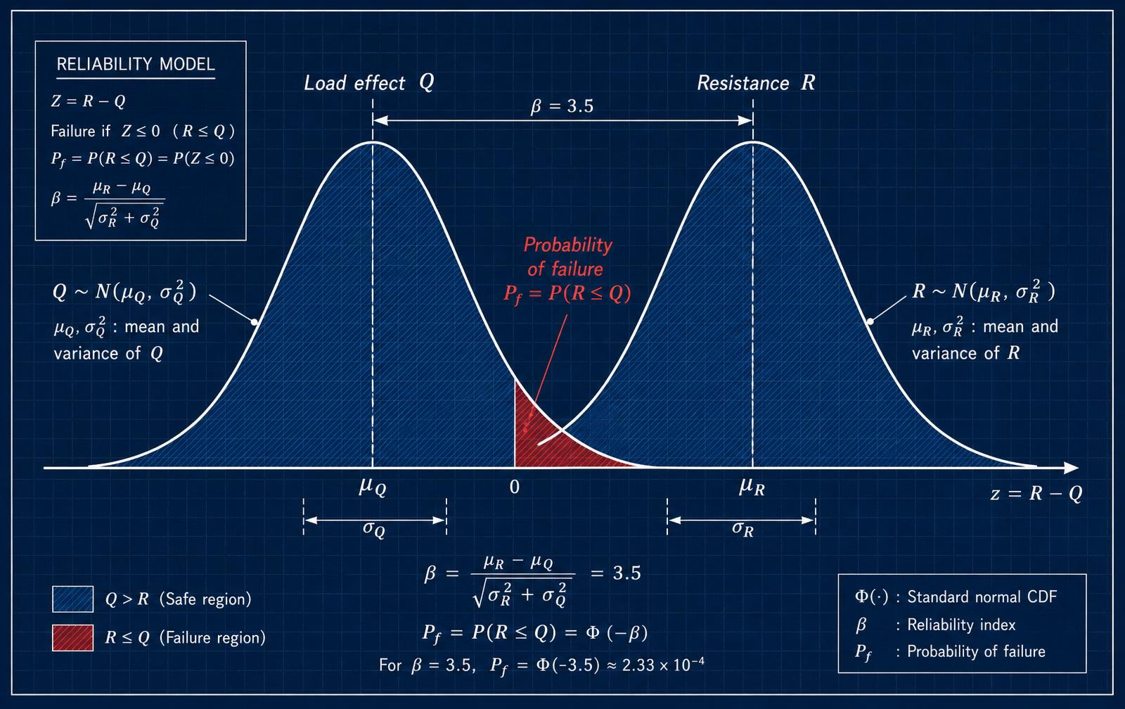
Calibrated for β ≈ 3.5

AASHTO LRFD was calibrated against a target reliability index β ≈ 3.5 at the Strength I limit state, corresponding to a failure probability of roughly 2×10⁻⁴ over the 75-year design life. β is the distance, in standard deviations, between the mean values of resistance R and load effect Q:

Formula
$\beta \;=\; \frac{\mu_{R} - \mu_{Q}}{\sqrt{\sigma_{R}^{2} + \sigma_{Q}^{2}}}$

$\mu_{R}$: mean of resistance R
$\mu_{Q}$: mean of load effect Q
$\sigma_{R},\ \sigma_{Q}$: standard deviations of R and Q

Overlapping normal distributions of load effect Q and resistance R with shaded probability-of-failure region and reliability index beta annotation — Figure 2.3Load–resistance reliability model. LRFD calibration positions the mean resistance μR far enough above the mean load effect μQ that the standard-normal exceedance probability P(R ≤ Q) = Φ(−β) reaches the target reliability. AASHTO LRFD adopts β ≈ 3.5 → Pf ≈ 2×10⁻⁴ over 75 years.

AASHTO LRFD Reference

Any resistance model modified outside of AASHTO must be independently re-calibrated to the same β target before use in production design. Cite the calibration study explicitly.

2.10 — Design live load

HL-93

AASHTO LRFD §3.6.1.2

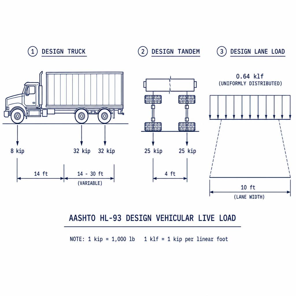
HL-93 is a notional live load where H represents the HS truck, L the lane load, and 93 the year the load was adopted. It consists of a combination of:

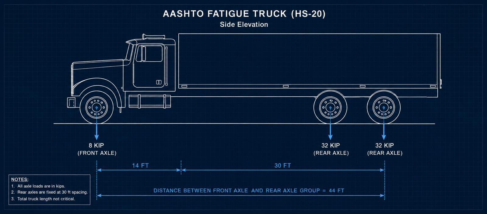
Design truck (HS-20): 8 kip front axle, two 32 kip rear axles at 14 ft and 14–30 ft (variable) spacing.
Design tandem: a pair of 25 kip axles spaced 4 ft apart.
Design lane load: 0.64 kip/ft uniformly distributed longitudinally, occupying a 10-ft-wide strip within a 12-ft design lane. The lane load is not subject to dynamic allowance.

The transverse spacing of wheels for both the design truck and design tandem is 6.0 ft. The uniform lane load may be continuous or discontinuous, as necessary to produce the maximum force effect.

AASHTO HL-93 design truck, design tandem, and design lane load configurations — Figure 2.4AASHTO HL-93 live-load configurations. Design demand at any location is the maximum of (truck + lane) and (tandem + lane), each amplified by the dynamic load allowance IM applied only to the truck / tandem.

2.11 — Fatigue live load

Single truck, 30-ft fixed spacing

AASHTO LRFD §3.6.1.4

The fatigue live load consists of a single design truck with the rear axle group fixed at 30 ft spacing between the 32 kip axles. The frequency of the fatigue load is taken as the single-lane average daily truck traffic (ADTT_SL). When the bridge is analyzed by approximate load distribution (§4.6.2), the single-lane distribution factor is used.

Side elevation of the AASHTO fatigue truck showing 8-kip front axle and two 32-kip rear axles at fixed 30-ft spacing — Figure 2.5AASHTO fatigue truck (§3.6.1.4). Total axle load = 72 kips; rear-axle spacing fixed at 30 ft. Applied with γ = 1.75 for infinite-life (Fatigue I) or γ = 0.80 for finite-life (Fatigue II) checks.

2.12 — Number of design lanes

NL

AASHTO LRFD §3.6.1.1.1

Formula
$N_{L} \;=\; \text{INT}\!\left(\tfrac{w}{12}\right)$

$N_{L}$: number of design lanes (integer)
$w$: clear roadway width (curb-to-curb) [ft]

Example: for w = 40 ft, N_L = INT(40/12) = 3 design lanes. Roadways from 20 to 24 ft carry two design lanes each equal to half the roadway width.

2.13 — Multiple presence factor

m

AASHTO LRFD §3.6.1.1.2

Number of loaded lanes	Multiple-presence factor, m
1	1.20
2	1.00
3	0.85
> 3	0.65

Table 2.5 — AASHTO Table 3.6.1.1.2-1. m reflects the reduced probability that multiple lanes are simultaneously loaded to full HL-93 magnitude. When approximate live-load distribution factors are used, m is already embedded and shall not be applied again.

2.14 — Dynamic load allowance

IM

AASHTO LRFD §3.6.2

Component	IM (%)
Deck joints — all limit states	75%
All other components — fatigue and fracture limit states	15%
All other components — all other limit states	33%

Table 2.6 — AASHTO Table 3.6.2.1-1. IM is applied to the design truck / tandem only and not to the design lane load. It also does not apply to pedestrian, wind, or centrifugal loads.

For bridges with reduced truck volume, AASHTO permits a fatigue-life adjustment based on single-lane average daily truck traffic: ADTT_SL < 1,000 → 95%; ADTT_SL < 100 → 90%. This reflects the reduced probability of attaining the design event during the 75-year reference period.

2.15 — Live-load distribution factors

DF for beam/girder bridges

AASHTO LRFD §4.6.2.2

Distribution factors (DF) convert lane demand into per-girder demand. AASHTO provides closed-form approximate equations, tabulated by cross-section type (steel/PS I-girder, box, T-beam, etc.), for both moment and shear, and separately for one-lane and multiple-lanes loaded, interior and exterior girders:

DFM_si — single-lane, interior beam, moment
DFM_mi — multiple-lane, interior beam, moment
DFM_se — single-lane, exterior beam, moment
DFM_me — multiple-lane, exterior beam, moment
DFV_si, DFV_mi, DFV_se, DFV_me — analogous for shear

DF is most sensitive to beam (girder) spacing; span length and longitudinal stiffness have smaller influences. Per AASHTO §2.5.2.7.1, the load-carrying capacity of an exterior beam shall not be less than that of an interior beam. Chapter 3 works through the DF calculation on the Maryland worked example.

2.16 — Strength I combination in practice

Assembling the demand

Worked demand — girder midspan moment

Given unfactored midspan moments M_DC = 620 k-ft, M_DW = 95 k-ft, M_LL+IM = 780 k-ft (already multiplied by distribution factor and IM):

M_u,Str-I = 1.00 × [ 1.25 × 620 + 1.50 × 95 + 1.75 × 780 ]
M_u,Str-I = 1.00 × [ 775.0 + 142.5 + 1,365.0 ] = 2,282.5 k-ft

This factored demand M_u must satisfy M_u ≤ φ M_n, with φ = 0.90 for reinforced concrete flexure or φ = 1.00 for prestressed concrete flexure. Chapter 3 walks through the full sequence — including how M_LL+IM was obtained — on the three-span Maryland bridge worked example.

Chapter summary

Key takeaways

LRFD balances calibrated load and resistance factors against a target β ≈ 3.5.
Four families of limit states — Strength, Service, Fatigue, Extreme Event — cover every design check.
η captures ductility, redundancy, and importance — usually 1.0 for standard bridges.
Permanent-load γp values (Table 3.4.1-2) differ for max vs. min effects; always pick the more critical.
HL-93 = larger of (design truck, design tandem) + design lane load; IM applies only to the truck / tandem.
Fatigue truck has fixed 30-ft rear-axle spacing; frequency = single-lane ADTT.
Multiple-presence factor m adjusts for the probability of simultaneous multi-lane loading.
DF depends most on girder spacing; exterior girders may never be weaker than interior.

Section 2

Fully Worked Examples

Complete AASHTO LRFD solutions with knowns, assumptions, step calculations, verification, and design commentary. Difficulty rises from basic to consulting-grade.

Worked Example 1

Compute a Strength I factored load effect

Basic

Problem

Compute the factored moment M_u under Strength I with η = 1.00.

Step-by-Step

\gamma _{DC} = 1.25 (max), \gamma _{DW} = 1.50, \gamma _{LL} = 1.75 for Strength I.

M_{u} = 1.00\cdot [1.25(0.90) + 1.50(0.25) + 1.75(5.60)]

Result

M_{u} = 1.125 + 0.375 + 9.80 = 11.30 k\cdot ft/ft

Design Verification

LL dominates (≈87%). This is normal for deck strips — deck design is nearly always live-load-controlled.

Discussion

The order 'multiply first, then sum' is essential — combining unfactored loads first and factoring the total is a common student error that hides which limit state governs.

Worked Example 2

Choose between Strength I and Strength IV for a long-span dead-load-dominated section

Intermediate

Problem

Determine the governing Strength limit-state axial force P_u.

Step-by-Step

P_{u} = 1.25(4200) + 1.75(320) = 5250 + 560

Result

5810 kip

P_{u} = 1.50(4200) + 0 = 6300 kip

Result

6300 kip

Design Verification

Strength IV activates when the DC/(LL+IM) ratio is high (~7×). Here 4200/320 ≈ 13, well past the trigger. ✓

Discussion

Truss chords and long-span girders routinely see Strength IV govern. On short spans, Strength I almost always controls.

Worked Example 3

Reliability index check on a bearing pad

Advanced

Problem

Verify Strength I demand vs φR_n and comment on the implied reliability index β.

Step-by-Step

Q_{u} = 1.25(45) + 1.75(55) = 56.25 + 96.25

Result

Q_{u} = 152.5 kip

\phi R_{n} = 1.00(180)

Result

180 kip

Design Verification

Utilization 0.85 leaves a 15% margin above the calibration target β = 3.5 (Pf ≈ 1 in 4300).

Discussion

LRFD does not compute β for you — it embeds it in the γ/φ pair. Utilization > 1 means either β falls below 3.5 or a redistribution is required.

Worked Example 4

Fatigue I load combination on a welded stiffener detail

Intermediate

Problem

Verify infinite-life fatigue per Fatigue I load combination (γ_LL = 1.75).

Step-by-Step

\Delta f_{IM} = (1+IM)\,\Delta f = 1.15\,(3.2) = 3.68\ \text{ksi}

\gamma_{LL}\,\Delta f_{IM} = 1.75\,(3.68)

Result

\Delta f_{\text{eff}} = 6.44\ \text{ksi}

Design Verification

Utilization 6.44/12 = 0.54 — comfortable margin. If the detail had been Cat E′ ((ΔF)_TH = 2.6 ksi), the same Δf would fail decisively.

Discussion

Fatigue I (γ = 1.75) targets infinite life; Fatigue II (γ = 0.80) targets finite life on low-ADTT structures. Never mix load factors between checks — pick the combination that matches the design life goal.

Worked Example 5

Service III tension check at a PS girder bottom fiber

Advanced

Problem

Verify Service III (γ_LL = 0.80) tension limit for prestressed concrete.

Step-by-Step

\sigma_{bot} = \sigma_{pe} + \sigma_{DC} + \gamma_{LL}\,\sigma_{LL+IM}

\sigma_{bot} = -2.80 + (-1.20) + 0.80\,(+0.90)

Result

\sigma_{bot} = -3.28\ \text{ksi\ (compression)}

Design Verification

The section stays in compression at Service III; no crack initiation is expected under characteristic live load.

Discussion

Service III uses γ_LL = 0.80 because the tension limit is calibrated to a lower live-load fractile — the goal is crack control, not strength. Applying γ_LL = 1.00 here would over-penalize prestressed girders.

Section 3

Guided Practice

Complete the missing steps. Use Hints for AASHTO article pointers and setup logic before revealing the full step. Submit at the end to send your work to your instructor.

Guided Problem 1

Strength I demand for an interior girder

A simply supported interior prestressed I-girder has these unfactored moments at midspan: $M_{DC}=1{,}050$ k-ft (girder + deck), $M_{DW}=180$ k-ft (2-in future overlay), and a per-lane truck live-load moment $M_{LL}^{\text{lane}}=960$ k-ft (no impact). The distribution factor is $g=0.55$ and IM = 33%.

Assemble the Strength I moment M_u with η = 1.0.

Step 1Distributed live-load moment per girder:

M_{LL}^{\text{gir}} = g\,M_{LL}^{\text{lane}}

(k-ft).

Answer (k-ft)

Step 2Include impact:

M_{LL+IM} = (1+IM)\,M_{LL}^{\text{gir}}

(k-ft).

Answer (k-ft)

Step 3Strength I moment:

M_u = 1.25 M_{DC} + 1.50 M_{DW} + 1.75 M_{LL+IM}

(k-ft).

Answer (k-ft)

Guided Problem 2

Load modifier η for a fracture-critical steel girder

A two-girder steel bridge is nonredundant (both girders are fracture-critical), the weld detail is not enhanced-ductility, and the bridge carries a designated emergency route.

Compute η for use in Strength I where γ is taken at its maximum value.

Step 1Ductility factor

\eta_D

per §1.3.3.

Answer

Step 2Redundancy factor

\eta_R

per §1.3.4.

Answer

Step 3Importance factor

\eta_I

per §1.3.5.

Answer

Step 4Combined load modifier

\eta = \eta_D\,\eta_R\,\eta_I \ge 0.95

Answer

Guided Problem 3

Design lanes and multiple-presence for a 3-lane fill

A rural bridge has a clear roadway w = 38 ft. Two lanes of AASHTO design trucks each produce a girder moment M₁ = 720 k-ft (per lane, per girder, no impact) using the appropriate distribution factor. Include IM = 33%.

Determine N_L, choose the correct multiple-presence factor m, and compute the Service I contribution of live load per girder.

Step 1Number of design lanes

N_L = \lfloor w/12 \rfloor

Answer

Step 2Multiple-presence factor m for 2 loaded lanes (design controlling case).

Answer

Step 3Live-load-plus-impact moment per girder with two lanes acting:

M_{LL+IM} = m\,(1+IM)\,(M_1 + M_2)

, taking M₁ = M₂ = 720 k-ft (k-ft).

Answer (k-ft)

Guided Problem 4

Fatigue I check on a steel welded detail

A Category C′ transverse stiffener-to-web weld on a plate girder sees a fatigue-truck stress range Δf = 4.2 ksi (from a single fatigue truck, before load factor and impact). IM for fatigue = 15%. The infinite-life threshold for Category C′ is $(\Delta F)_{TH} = 12$ ksi.

Check the Fatigue I stress range and decide whether the detail meets the infinite-life criterion.

Step 1Fatigue I stress range:

\gamma\,(1+IM)\,\Delta f = 1.75(1.15)\Delta f

(ksi).

Answer (ksi)

Step 2Ratio of Fatigue I demand to the infinite-life threshold for Category C′:

(\Delta f)/(\Delta F)_{TH}

Answer