
Engineering story
The Woodrow Wilson Bridge — a Mid-Atlantic loading lesson
The original Woodrow Wilson Bridge, carrying I-95/I-495 across the Potomac between Alexandria, Virginia and Prince George's County, Maryland, opened in 1961 for a projected 75,000 vehicles per day. By 2000 it carried more than 200,000 vehicles per day — a live-load environment far in excess of the loading assumptions used in its original 1950s design. A landmark FHWA and NCHRP investigation of the crossing (a driver behind the development of the HL-93 notional load model) documented growing fatigue damage, deck deterioration, and a rising fraction of permit trucks. It was demolished after the replacement twin bascule bridges opened in 2006–2008.

The Woodrow Wilson replacement was designed to AASHTO LRFD and rated for HL-93 plus MDOT SHA / VDOT permit envelopes. That project — plus MDOT SHA's ongoing evaluation of the Chesapeake Bay Bridge and the recovery of the Francis Scott Key Bridge site — illustrates why loads (not resistance) drive most modern bridge decisions in the Mid-Atlantic.
Heavily trafficked urban
American Legion Bridge (I-495 over the Potomac). ~230,000 vehicles/day; ongoing MDOT-Virginia joint replacement project driven by capacity and deck condition.
Rural interstate
I-70 over the South Branch, Washington County, MD. Governed by fatigue truck loading and future overlay assumptions rather than peak demand.
Permit-vehicle bridge
US 40 crossings routing MDOT SHA permit vehicles (superloads for wind-turbine components). Strength II combinations control the load rating.
Vessel-collision case
Francis Scott Key Bridge (I-695, 1977–2024). Container-vessel strike on a non-redundant pier caused progressive collapse — an extreme-event limit state failure.
Fatigue-governed detail
Girder-web welded stiffener terminations along US-50; MDOT SHA fatigue retrofits under §6.6.1 Category C details.
Chapter objectives
What you will be able to do
Learning objectives
By the end of this chapter you will be able to:
- 1Identify all permanent and transient loads that act on a highway bridge.
- 2Compute HL-93 live-load force effects for simple and continuous spans.
- 3Apply the correct dynamic load allowance IM and multiple-presence factor m.
- 4Select and compute Strength I, Service I, Fatigue I, and Extreme Event II combinations.
- 5Position design truck, tandem, and lane loads for maximum moment and shear using influence lines.
- 6Distinguish DC, DW, LL, IM, BR, WA, WS, WL, TU, EQ, CT, CV, CR, SH loads.
- 7Verify computed demands with independent hand checks and code-based envelopes.
- 8Interpret the permit-vehicle envelope adopted by MDOT SHA and neighboring DOTs.
Pre-lecture — Section properties & load computation
Before you compute demands: how a bridge cross-section actually resists load
Every demand you will compute in §3.1 – §3.8 is only meaningful when you also know the section that resists it. In a composite steel–concrete bridge the resisting section is not one section — it is three or four, depending on the age of the concrete, the direction of bending, and whether the deck is cracked. This pre-lecture builds the vocabulary and the arithmetic you need to turn a plate girder + deck sketch into a set of design section properties (A, I, Stop, Sbot) and then apply the correct permanent-load pieces (self-weight, deck, SIP formwork, haunch, barriers, wearing surface, cross-frames) at the correct sequence in construction.
Why the sequence matters
PL.1 — Terminology
Naming every piece of a composite bridge cross-section
Section properties are fundamental to load and stress computations, structural analysis, and resistance/capacity checks. In this course they include cross-sectional area A, centroid location ȳ, moment of inertia I, section modulus S, and slenderness ratios. Before we compute any of them, we need agreement on names.
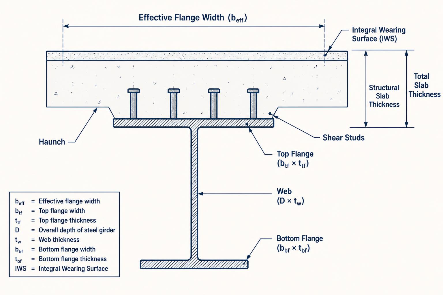
| Term | Definition | Typical value |
|---|---|---|
| Total slab thickness | Full deck depth as poured (IWS + structural). | 8 in – 9½ in |
| Integral Wearing Surface (IWS) | Sacrificial top layer of the deck assumed to wear off over the design life. | ¼ in – ½ in |
| Structural slab thickness | Deck depth remaining after IWS is deducted. Used for capacity. | 7½ in – 9 in |
| Haunch | Gap between top of steel web and underside of the deck. Accommodates screed elevation and formwork tolerance. | 2 in – 4 in |
| Effective flange width, b_eff | Portion of the deck that acts compositely with a given girder. | See §4.6.2.6 (AASHTO) |
| Top flange | Compression flange of a positive-moment section. Sized against local buckling. | b_tf × t_tf |
| Web | Vertical plate resisting shear. Slenderness limited by D/t_w. | D × t_w |
| Bottom flange | Tension flange in positive-moment regions; typically 1.5× top flange area. | b_bf × t_bf |
IWS split-use rule
PL.2 — Effective flange width
Why only part of the deck acts as a girder flange
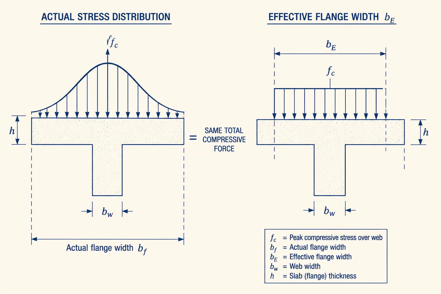
Concrete compression stress in a wide deck is highest directly above the girder web and drops off toward mid-span between girders — this is shear lag. Rather than integrate a curved stress block, AASHTO defines an effective flange width bE over which the peak stress fc is assumed uniform, delivering the same total compressive force.
AASHTO LRFD Reference
§4.6.2.6.1 — General. Unless specified otherwise, the effective flange width of a concrete deck slab in composite or monolithic construction may be taken as the tributary width perpendicular to the axis of the member for determining cross-section stiffnesses for analysis and for determining flexural resistances.
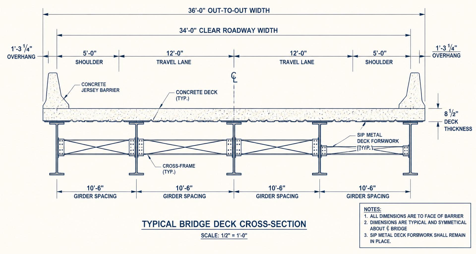
Tributary width means: for an interior girder, half the spacing to each adjacent girder — i.e. the full girder spacing S. For an exterior girder, half the spacing to the adjacent interior girder plus the deck overhang. That's why the same bridge often has two sets of composite section properties — one interior, one exterior. Always label your section with which one you are computing.
PL.3 — Materials & modular ratio
Transforming concrete into equivalent steel
The girder is steel and the deck is concrete — two materials with very different stiffnesses. To perform a single beam-bending analysis, we transform the concrete into an equivalent area of steel using the modular ratio n.
Modular ratio
- Modulus of elasticity of structural steel [ksi]
- Modulus of elasticity of concrete [ksi]
- Modular ratio, rounded to nearest whole number
For all grades of structural steel AASHTO AASHTO LRFD §6.4.1 sets Es = 29,000 ksi. For normal-weight concrete AASHTO AASHTO LRFD §C5.4.2.4 gives the practical form:
Concrete modulus
- Specified 28-day compressive strength [ksi]
| f′_c (ksi) | E_c (ksi) | n = 29,000 / E_c | Rounded n | 3n (long-term) |
|---|---|---|---|---|
| 3.0 | 3152 | 9.20 | 9 | 27 |
| 3.5 | 3405 | 8.50 | 8 | 24 |
| 4.0 | 3640 | 7.97 | 8 | 24 |
| 4.5 | 3861 | 7.51 | 8 | 24 |
| 5.0 | 4070 | 7.13 | 7 | 21 |
| 6.0 | 4458 | 6.51 | 7 | 21 |
| 8.0 | 5148 | 5.63 | 6 | 18 |
PL.4 — Positive-bending section family
Noncomposite, short-term composite, long-term composite
The class of section that resists a given load depends on when that load arrives on the bridge and how long it acts.
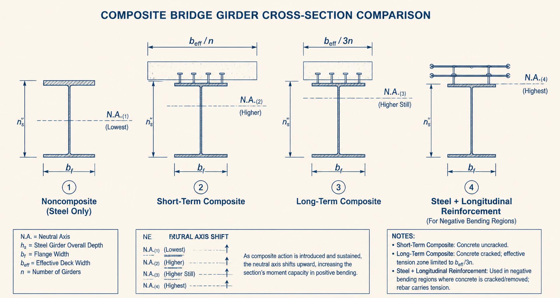
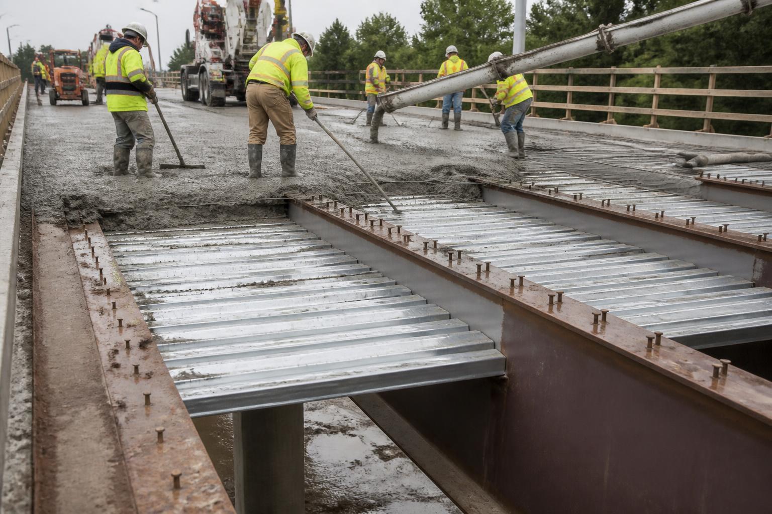
- Noncomposite (steel only). The bare steel girder — before the deck has cured — resists every load applied during construction: girder self-weight, wet concrete deck, haunch, SIP formwork, and cross-frames.
- Short-term composite (steel + b_eff / n). After the deck cures, transient loads (traffic, wind on live load) are applied for seconds to minutes. The concrete is transformed by dividing the effective width by n.
- Long-term composite (steel + b_eff / 3n). Permanent loads added after the deck cures — barriers, sidewalks, future wearing surface, utility conduits, sign structures — act for decades. Concrete creeps under sustained stress; using 3n instead of n reduces the transformed area so the steel picks up the extra strain the creeping concrete cannot sustain.
Why 3n and not 2n or 4n
PL.5 — Negative-bending sections
What happens over the pier
Over interior supports of continuous girders the top of the deck is in tension. Concrete has essentially no tensile strength for design purposes, so we assume the deck concrete cracks and take steel + longitudinal deck reinforcement as the resisting section. Two methods are permitted:
- Count every longitudinal deck bar within beff and include its area and centroid — tedious but exact.
- Use the conservative shortcut of AASHTO LRFD §6.10.1.1.1c: assume 1% longitudinal reinforcement in the effective flange width (two-thirds in the top mat, one-third in the bottom mat).
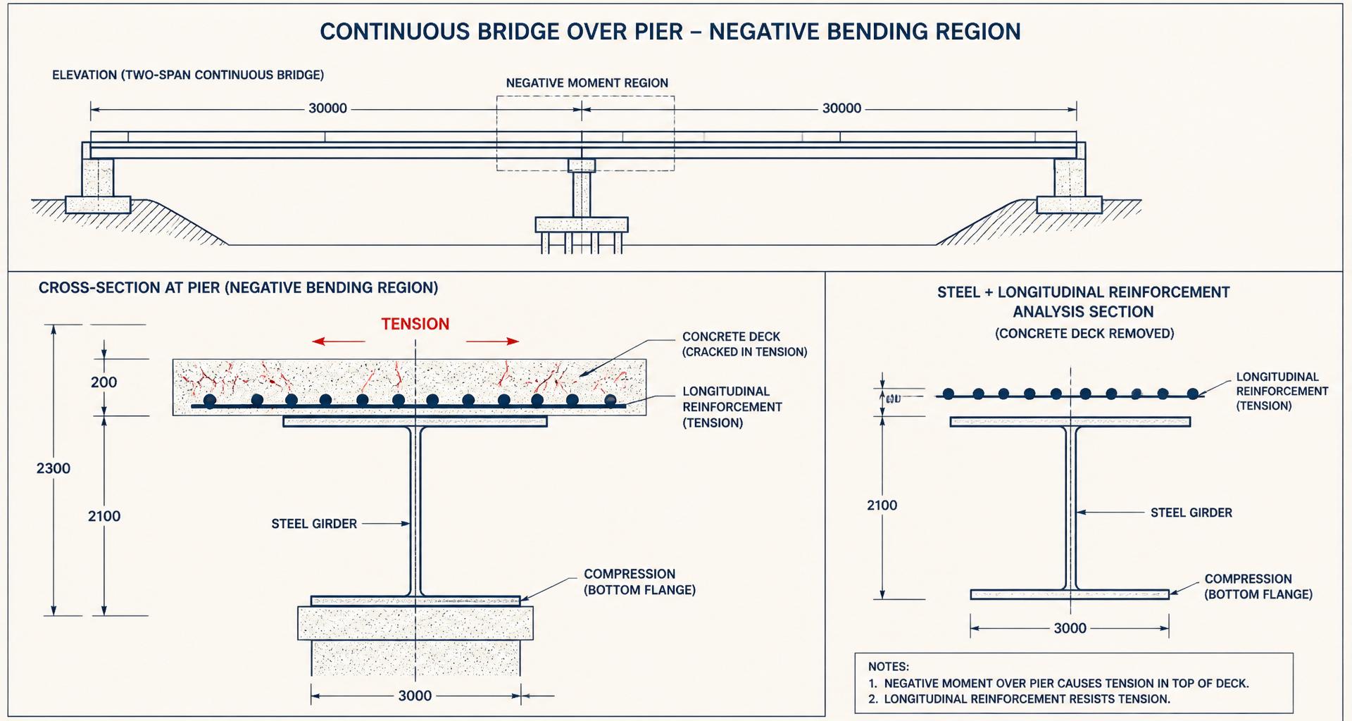
Design cover requirements (AASHTO §5.10.1)
PL.6 — The arithmetic
Parallel-axis theorem, applied to every section in the family
For each section variant (noncomposite, short-term, long-term, steel + rebar) you follow the same 5-step recipe:
- Choose a datum (usually bottom of bottom flange).
- List each component: area Ai and centroid height yi above the datum.
- Compute the section centroid ȳ = ΣAiyi / ΣAi.
- Compute each component's di = yi − ȳ, then sum I = Σ(Io,i + Aidi2).
- Get section moduli: Stop = I / ctop and Sbot = I / cbot.
Parallel-axis theorem
(PL.6-1)
Rectangle self-inertia
(PL.6-2)
Section modulus and bending stress
(PL.6-3)
PL.6b — Preliminary sizing
How to select a trial section for a plate girder
Before you can compute section properties you need a starting cross-section. The following rules come from AASHTO slenderness limits, plate-availability tables from the AASHTO/NSBA Steel Bridge Collaboration, and decades of fabricator practice. They give an economical trial girder — you will iterate once demands are known.
| # | Dimension | Code limit | Design rule (backed off) | Trial equation |
|---|---|---|---|---|
| 1 | Girder depth D | L/D ≤ 30 (Table 2.5.2.6.3-1) | L/D = 27.5 | D = L / 27.5 |
| 2 | Web thickness tw | D/t_w ≤ 150 (unstiffened) | D/t_w = 120 | t_w = D / 120 |
| 3 | Compression flange width bfc | b_f/D ≤ 1/6 | b_fc/D = 1/4 (stockier) | b_fc = D / 4 |
| 4 | Compression flange thickness tfc | b_fc/(2 t_fc) ≤ 0.38 √(E/F_yc) | Fy = 50 ksi → t_fc = b_fc/18.3 Fy = 70 ksi → t_fc = b_fc/15.5 | t_fc ≥ b_fc / (0.76 √(E/F_yc)) |
| 5 | Tension flange thickness tft | Typically 1.5× top flange | Assume b_ft = b_fc | t_ft = 1.5 t_fc |
Why these rules of thumb?
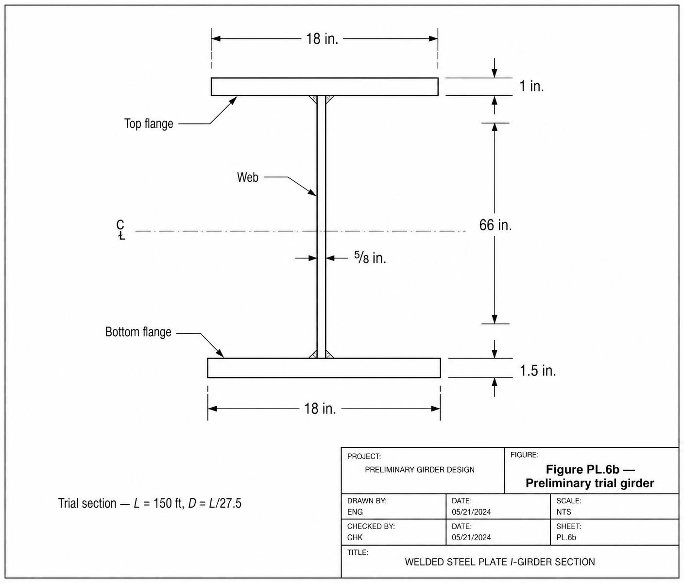
Worked trial — span L = 150 ft (1,800 in):
PL.6b
Trial section — span L = 150 ft (1,800 in)
Girder depth
Web thickness
Flange width
Flange thicknesses
Trial girder
Layout considerations before you draw plates
- Girder spacing. Wider is generally more economical (fewer girders, cross-frames, bearings). For L < 140 ft use S = 10–11 ft; for L > 140 ft use S = 11–14 ft. Wider spacing → thicker deck.
- Minimum plate thicknesses. Stiffeners & connection plates 7/16 in min (½ in preferred). Webs 7/16 in min (½ in preferred), 1/16-in increments. Flanges ¾ in min, 1/8-in increments up to 2½ in then ¼-in increments.
- Never change flange width along the girder — change thickness. Butt-weld thicker flange plates with CJP welds, torch-cut a 60-in min transition length. Constant flange width simplifies fabrication.
- Plate availability. Use AASHTO/NSBA plate-length tables (e.g. ½-in × 72-in plate available up to ~972 in long, 3-in × 96-in only ~734 in) so you don't specify a plate the mill can't roll.
PL.7 — Worked example
Noncomposite section properties of a 42-in plate girder
Compute ȳ, I, and both section moduli for the steel-only cross-section below. This is the section that resists deck-pour loading — before composite action develops.
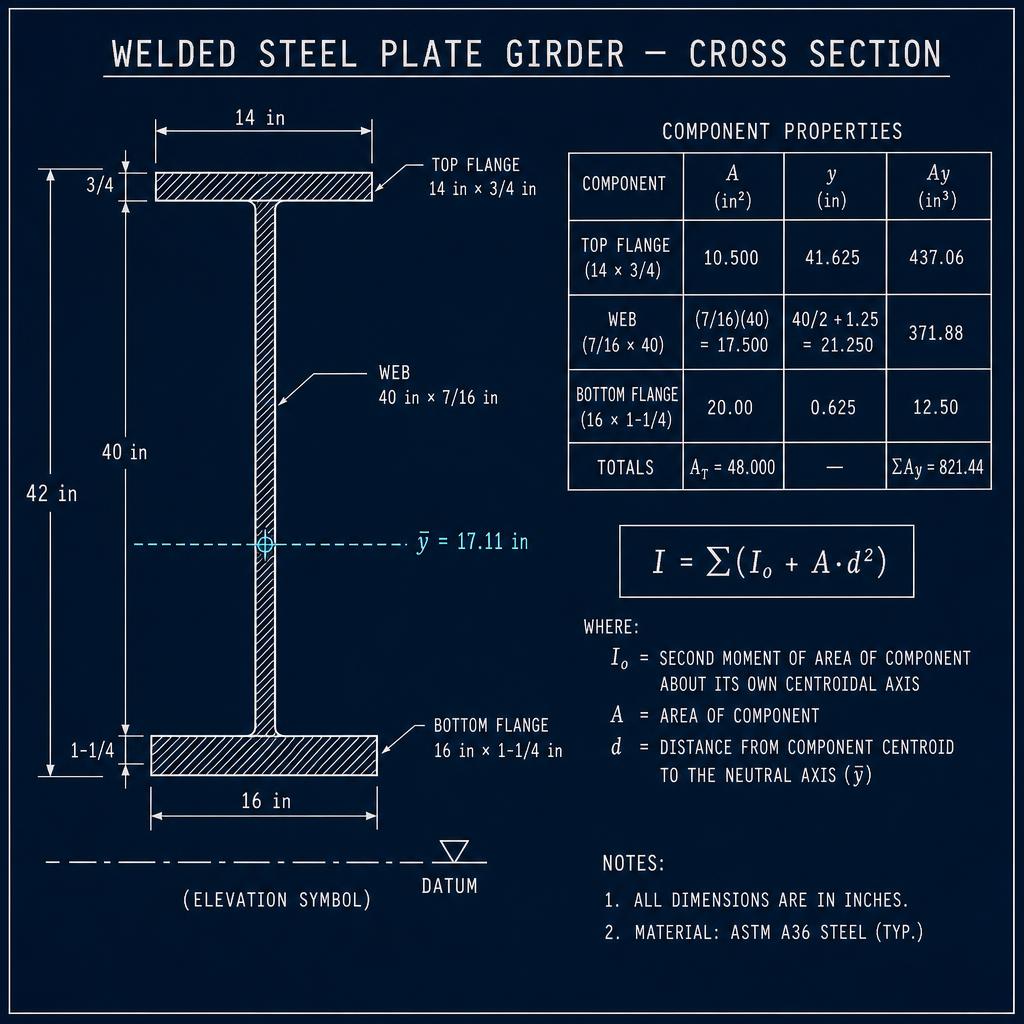
| Component | A (in²) | y (in) | Ay (in³) | I_o (in⁴) | d = y − ȳ (in) | Ad² (in⁴) |
|---|---|---|---|---|---|---|
| Top flange (14 × ¾) | 10.500 | 41.625 | 437.06 | 0.492 | +24.512 | 6,308.5 |
| Web (40 × 7/16) | 17.500 | 21.250 | 371.88 | 2,333.33 | +4.137 | 299.5 |
| Bottom flange (16 × 1¼) | 20.000 | 0.625 | 12.50 | 2.60 | −16.488 | 5,437.0 |
| Σ | 48.000 | — | 821.44 | 2,336.43 | — | 12,045.0 |
PL.7
Steel-only section properties (bare plate girder)
Centroid
Moment of inertia
Section modulus — top
Section modulus — bottom
Bare-steel properties
- centroid above the datum [in]
- second moment of area about the neutral axis [in^4]
- distance from neutral axis to extreme fibre [in]
Short-term composite — same recipe, one extra row
PL.8 — Permanent loads
What weighs on the bridge, and which section catches it
Permanent loads are grouped by which section resists them, because that drives the modular ratio used in analysis. AASHTO breaks the components into two design codes — DC (structural components and non-structural attachments) and DW (wearing surfaces and utilities) — because they carry different load factors (γp = 1.25/0.90 for DC vs. 1.50/0.65 for DW).
| Permanent load | Code | Applied to | Typical value | Formula per girder |
|---|---|---|---|---|
| Steel plate girder self-weight | DC1 | Noncomposite (steel only) | ρ_s = 490 pcf ≈ 0.490 kcf | w_g = A_s × ρ_s |
| Wet concrete deck (total thickness) | DC1 | Noncomposite (steel only) | ρ_c = 150 pcf; add 5 pcf for reinforcement → 155 pcf | w_deck = t_total × S × ρ_c |
| Concrete haunch | DC1 | Noncomposite (steel only) | 0.150 kcf × haunch height × top-flange width | w_h = t_haunch × b_tf × ρ_c |
| SIP metal deck formwork + ponded concrete in flutes | DC1 | Noncomposite (steel only) | ≈15 psf of deck area (form) + concrete fill (add ¼ in equivalent) | w_SIP = 15 psf × (S − b_tf) |
| Cross-frames / diaphragms | DC1 | Noncomposite (steel only) | Point loads at brace lines; ~200 – 500 lb each end reaction | Distribute to nearest node |
| Stiffeners, splice plates, bolts | DC1 | Noncomposite (steel only) | 5 – 10% uplift on girder self-weight | w_misc = 0.08 × w_g |
| Concrete parapets / Jersey barriers | DC2 | Long-term composite (3n) | MDOT SHA F-shape ≈ 470 plf per barrier | w_b = (Σ barriers) / N_g (or distribute to exterior only) |
| Sidewalks / raised medians (if cast after deck) | DC2 | Long-term composite (3n) | 0.150 kcf × sidewalk cross-section | w_sw = A_sw × ρ_c / N_g |
| Bituminous wearing surface / future overlay | DW | Long-term composite (3n) | MDOT SHA: 25 – 30 psf (2-in asphalt) | w_ws = t_ws × ρ_asp × (roadway width) / N_g |
| Utilities (waterline, gas, conduit) | DW | Long-term composite (3n) | Project-specific; get value from utility drawings | w_u = (weight per foot) / N_g |
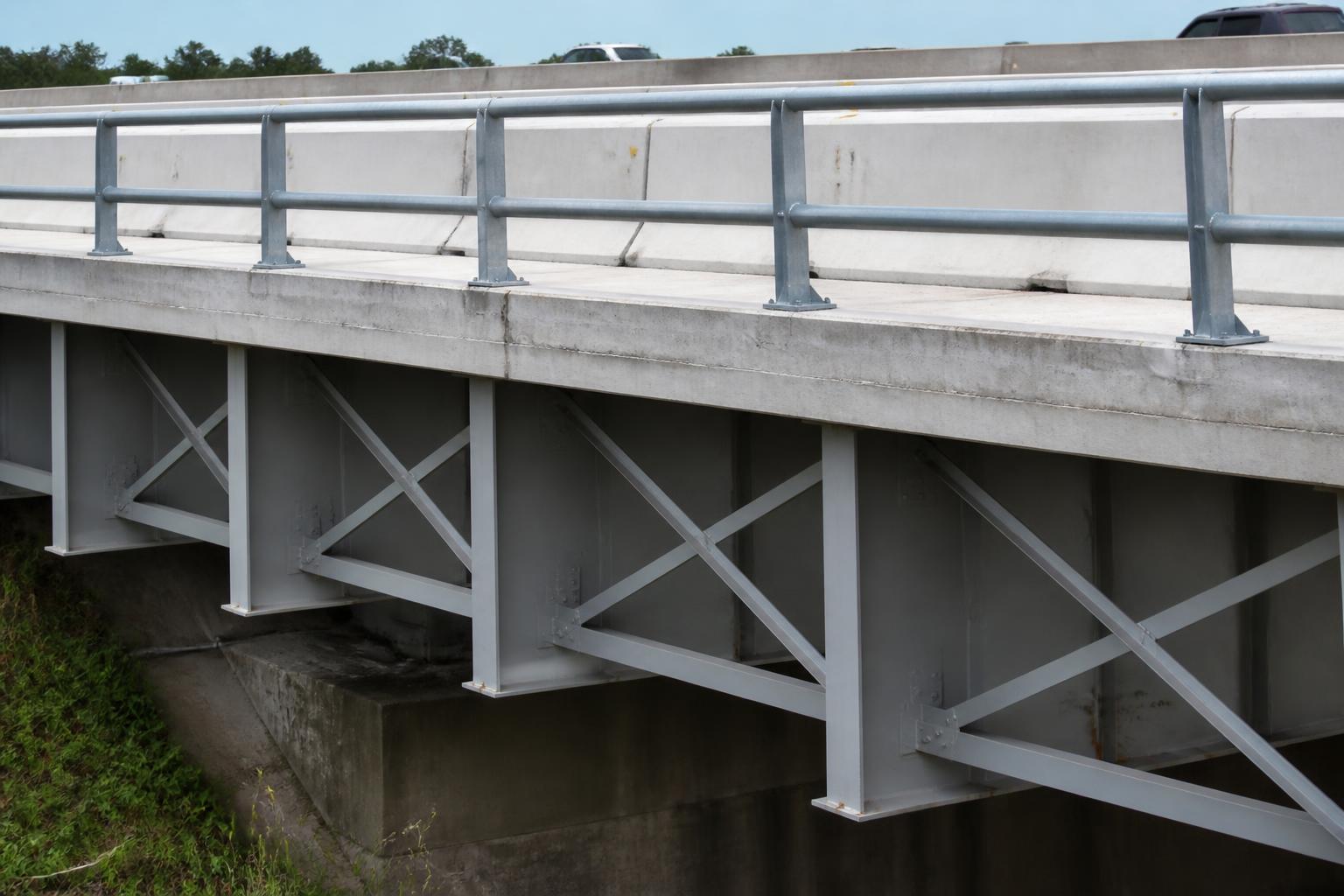
Distribution to girders
PL.8b — Worked example
Computing every permanent load on an interior girder
Given the bridge cross-section of Figure PL.4 (out-to-out width 36 ft, four girders at S = 10 ft 6 in, deck total ttotal = 8½ in with ½-in IWS, haunch = 2 in, top flange btf = 14 in, two F-shape barriers) and the trial girder from §PL.6b (As = 48.875 in²), compute the DC1, DC2, and DW loads carried by one interior girder. Use ρc = 0.150 kcf and ρs = 0.490 kcf.
Step 1 — DC1: steel girder self-weight
Formula
Substitute
Result
Add ~8% for stiffeners, splices, connection plates:
Formula
Result
Step 2 — DC1: wet concrete deck
Formula
Substitute
Result
Step 3 — DC1: haunch
Formula
Substitute
Result
Step 4 — DC1: SIP formwork + concrete in flutes
Take 15 psf of the tributary form area (girder spacing minus top flange width):
Formula
Substitute
Result
Step 5 — DC1: cross-frames (as an equivalent UDL)
Assume K-frames at 25-ft spacing, each weighing ~350 lb; end reaction on one girder ~175 lb. Smeared over 25 ft:
Substitute
Result
| DC1 component | w (klf) |
|---|---|
| Steel girder + details | 0.180 |
| Wet concrete deck | 1.116 |
| Haunch | 0.029 |
| SIP formwork + fill | 0.140 |
| Cross-frames (smeared) | 0.007 |
| Σ wDC1 | 1.472 klf |
Applied to the noncomposite steel section.
Step 6 — DC2: barriers
Two F-shape barriers at 0.470 klf each, distributed equally to the four girders:
Substitute
Result
Step 7 — DW: future wearing surface
Assume 25 psf over the 34-ft clear roadway, distributed to all four girders:
Substitute
Result
| Applied later | Code | w (klf) | Resisting section |
|---|---|---|---|
| Barriers | DC2 | 0.235 | Long-term composite (3n) |
| Future wearing surface | DW | 0.213 | Long-term composite (3n) |
Sanity check the numbers
PL.9 — Live loads, at a glance
What §3.1 – §3.4 will compute for you
The three live-load streams you will meet in §3.2 are all resisted by the short-term composite section:
- HL-93 design truck (8 + 32 + 32 kip axles) — see §3.2.
- HL-93 design tandem (25 + 25 kip axles, 4 ft apart) — governs short spans.
- Design lane load (0.64 klf uniform) — the "traffic queue" component, always superimposed on truck or tandem.
Each is amplified by the dynamic load allowance IM (33% for strength, 15% for fatigue) and factored for how many lanes are simultaneously loaded via the multiple-presence factor m. Finally, an approximate live-load distribution factor DF (AASHTO Table 4.6.2.2.2b-1) assigns a fraction of the axle line to each girder — because you almost never do a full 3D analysis for routine composite steel bridges.
Live-load moment
With MLL+IM in hand and SST from §PL.7 you can already compute the live-load bending stress at any fiber:
Bending stress
…which you'll then combine with the DC1 stress (on noncomposite S) and DC2 + DW stresses (on long-term S) in the Strength I equation from §3.4.
PL.10 — Design workflow
Putting section properties + loads together
- Sketch the cross-section with dimensions. Note interior vs exterior girder, spacing, overhang, deck thickness, IWS, haunch.
- Compute the noncomposite section properties (§PL.7 recipe).
- Compute beff (§PL.2), then the short-term composite (÷n) and long-term composite (÷3n) properties.
- For continuous spans, also compute the steel + longitudinal reinforcement properties for negative-moment regions (§PL.5).
- List every permanent load (§PL.8) and tag it DC1 / DC2 / DW. Compute its unfactored moment/shear per girder using structural analysis (Chapter 4 tools).
- Compute the live-load force effects (§3.2 – §3.3) and apply the distribution factor.
- Combine with the AASHTO load factors from Table 3.4.1-1 (§3.4). Check stresses on the correct section for each load type.
Common mistakes to avoid
- Using short-term S for the barrier or the future wearing surface.
- Forgetting the haunch weight (it can be 20 – 40 plf per girder).
- Forgetting SIP formwork (~15 psf) — often 5 – 10% of the deck DC1.
- Using total slab thickness for capacity or structural slab thickness for weight.
- Using interior beff for both interior and exterior girders.
- Dividing barrier weight by the number of girders when only the exterior girder should carry it.
With this pre-lecture complete you're ready for §3.1 Load Categories (below), where we formalize the AASHTO notation for every load type you just met, and then move into the HL-93 live-load model, dynamic allowance, and Strength/Service combinations.
3.1 — Load categories
Permanent, transient, extreme
Every highway bridge is subject to two broad classes of loads: permanent (present throughout the design life, essentially constant) and transient (variable in space, time, or occurrence). AASHTO LRFD subdivides these into notation each engineer must memorize, because every subsequent chapter references it.
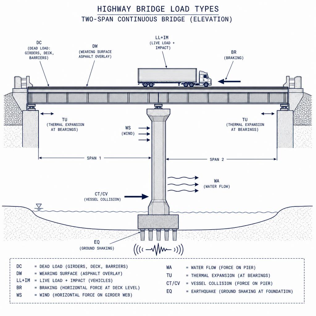
| Notation | Name | Typical source |
|---|---|---|
| DC | Dead load of components + attachments | Girders, deck, diaphragms, barriers |
| DW | Dead load of wearing surface + utilities | Asphalt overlay, waterline, conduit |
| EH / EV / ES | Earth pressure (horizontal / vertical / surcharge) | Backfill on abutments and walls |
| LL | Vehicular live load | HL-93 truck, tandem, lane |
| IM | Dynamic load allowance | Impact factor applied to LL truck/tandem |
| BR | Vehicular braking force | Decelerating trucks |
| CE | Vehicular centrifugal force | Curved bridges |
| PL | Pedestrian load | Sidewalks > 2 ft |
| WA | Water load & stream pressure | Piers in waterway |
| WS / WL | Wind on structure / wind on live load | Girder web, deck overhang |
| TU / TG | Uniform thermal / thermal gradient | Bearings, expansion joints, continuous frames |
| CR / SH | Creep / shrinkage | Time-dependent PC girder behavior |
| EQ | Earthquake | Seismic design |
| CT / CV | Vehicular / vessel collision | Piers exposed to traffic or navigation |
| IC | Ice load | Northern rivers |
Estimating dead load (DC, DW). Dead load of a structural component is its volume times its unit weight. AASHTO LRFD Table 3.5.1-1 tabulates the unit weights the designer must use so that every engineer computing DC and DW on the same girder arrives at the same number. The most-used values are reproduced below (kip/ft³):
| Material | Unit weight γ (kip/ft³) | Where it appears |
|---|---|---|
| Normal-weight concrete (f′c ≤ 5 ksi, incl. reinforcement) | 0.145 | Deck, girder, pier, abutment (DC) |
| Normal-weight concrete (5 < f′c < 15 ksi) | 0.140 + 0.001·f′c | High-strength PC girders (DC) |
| Lightweight concrete (incl. reinforcement) | 0.110 | Deck on long-span steel (DC) |
| Sand-lightweight concrete (incl. reinforcement) | 0.120 | Deck (DC) |
| Structural steel | 0.490 | Plate girders, rolled beams (DC) |
| Cast iron | 0.450 | Legacy bridges (DC) |
| Aluminum | 0.175 | Signs, luminaires (DC) |
| Bituminous wearing surface (asphalt) | 0.140 | Future overlay (DW) |
| Stone masonry | 0.170 | Historic arch spandrels, retaining (DC) |
| Hardwood / softwood | 0.060 / 0.050 | Timber decks, formwork |
| Water (fresh / salt) | 0.062 / 0.064 | Buoyancy on submerged piers (WA) |
| Compact sand, silt, or clay | 0.120 | Backfill above abutment footings (EV) |
| Loose sand, silt, or gravel | 0.100 | Backfill (EV) |
| Transit rails, ties & fastenings | 0.200 kip/ft (per track) | Rail transit deck loads (DC) |
Adapted from AASHTO LRFD §3.5.1 (Table 3.5.1-1), 10th Edition (2024). Verify current values against the specification for each new design; older editions used slightly different concrete-strength thresholds.
Why DC and DW carry different load factors
3.1.5 — Load-by-load lecture
How each highway-bridge load is quantified
The table above lists the notation; this lecture is what the notation actually means in a design calculation. For each load, you need to know (a) the physical mechanism, (b) the AASHTO-prescribed equation or table used to quantify it, and (c) the units and typical magnitude on a Mid-Atlantic bridge. Every worked example in this course draws from the equations below.
DC — Dead load of structural components AASHTO LRFD §3.5.1
The self-weight of everything that forms part of the structure: girders, deck slab, diaphragms, cross-frames, stiffeners, bearings, barriers, and end blocks. Computed by multiplying volume by unit weight from AASHTO Table 3.5.1-1 (γc = 150 pcf for normal-weight reinforced concrete, γs = 490 pcf for structural steel).
Example: a 9-in cast-in-place deck at 10-ft girder spacing gives wDC,deck = 0.150 · 0.75 · 10 = 1.125 klf on each interior girder.
DW — Dead load of wearing surface and utilities AASHTO LRFD §3.5.1
Everything not part of the structural cross-section: asphalt overlay, waterproofing membrane, utilities (waterlines, conduits, gas lines). DW is separated from DC because it has a higher load factor (γDW = 1.50 vs. γDC = 1.25) — future overlays and utilities are far less certain than the structural steel weight.
MDOT SHA standard future-wearing-surface allowance: qFWS = 0.025 ksf (equivalent to a 2-in bituminous overlay at 150 pcf).
LL — Vehicular live load AASHTO LRFD §3.6.1
HL-93 as introduced in §3.2. The force effect from LL is obtained by positioning the design truck (or tandem) and design lane load on the influence line for the response of interest. A closed-form simple-span expression that every graduate should have memorized:
Lane load moment
Truck moment (simple span)
Depends on rear-axle spacing
BR — Vehicular braking force AASHTO LRFD §3.6.4
Horizontal force at 6 ft above the deck, applied longitudinally to the superstructure to represent decelerating trucks. AASHTO requires the larger of:
Multiple-presence factor m applies to BR.
WA — Water load and stream pressure AASHTO LRFD §3.7
Longitudinal pressure on a pier submerged in flowing water:
C_D = drag coefficient (0.7 for semicircular nose, 1.4 for square).
WS — Wind on structure AASHTO LRFD §3.8
The 10th Edition adopts the same wind-hazard framework used by ASCE 7 (basic wind speed V, exposure category, gust factor, pressure coefficients). Design pressure on the exposed area of the girder web and barriers:
TU — Uniform thermal expansion AASHTO LRFD §3.12.2
Change in bridge length due to uniform temperature change; drives bearing displacement and pier flexure. For Maryland (moderate climate zone, cold-climate steel bridges): ΔT = 150 °F design range for steel and ΔT = 80 °F for concrete.
α_steel = 6.5 × 10⁻⁶ /°F; α_concrete = 6.0 × 10⁻⁶ /°F.
EQ — Earthquake AASHTO LRFD §3.10
Elastic seismic response coefficient Csm as a function of site class, SDS, SD1, and structural period T:
Maryland is a low-to-moderate seismic region; most MDOT SHA bridges fall in Seismic Zone 1 (SD1 ≤ 0.15) — minimum detailing requirements apply but explicit seismic analysis rarely governs member sizes.
CV / CT — Vessel or vehicle collision AASHTO LRFD §3.14
Extreme-event load on piers exposed to navigable waterways or highway traffic. Vessel impact force is a function of vessel dead-weight tonnage, transit speed, and pier geometry — the 2024 Francis Scott Key Bridge collapse is the reference case for the Mid-Atlantic and has driven MDOT SHA's revised vessel-collision risk assessments on the Bay and Patapsco crossings.
CR / SH — Creep and shrinkage AASHTO LRFD §5.4.2.3
Time-dependent volume changes in concrete. Critical for prestressed girders because they cause loss of prestress and long-term camber growth. Handled in detail in Chapter 9.
Concept checkpoint
For an interior girder of a straight 120-ft simple-span steel bridge in Baltimore County, rank the following demands from largest to smallest in Strength I:
(a) LL + IM (b) DC (c) DW (d) BR (e) WS. Typical answer: LL+IM > DC > DW ≫ WS ~ BR. Strength I omits WS entirely.
3.2 — HL-93
The design vehicular live load
HL-93 is a notional loading — its combination of design truck and design lane load was calibrated by NCHRP Project 12-33 to envelope the force effects of a fleet of real heavy vehicles observed on U.S. bridges. The design engineer selects, for each response of interest:
- (design truck + design lane load), or
- (design tandem + design lane load),
whichever produces the larger force effect.
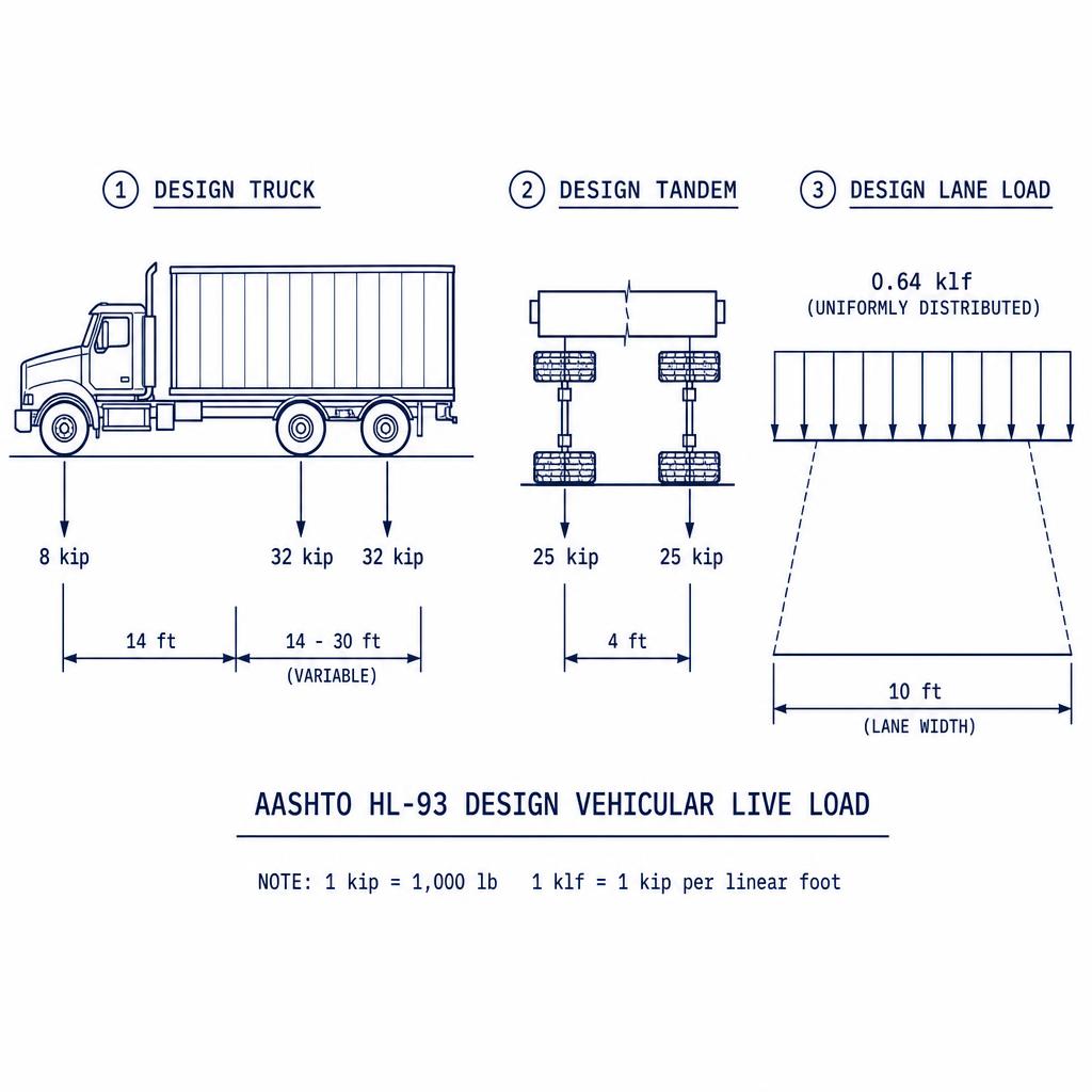
Design truck
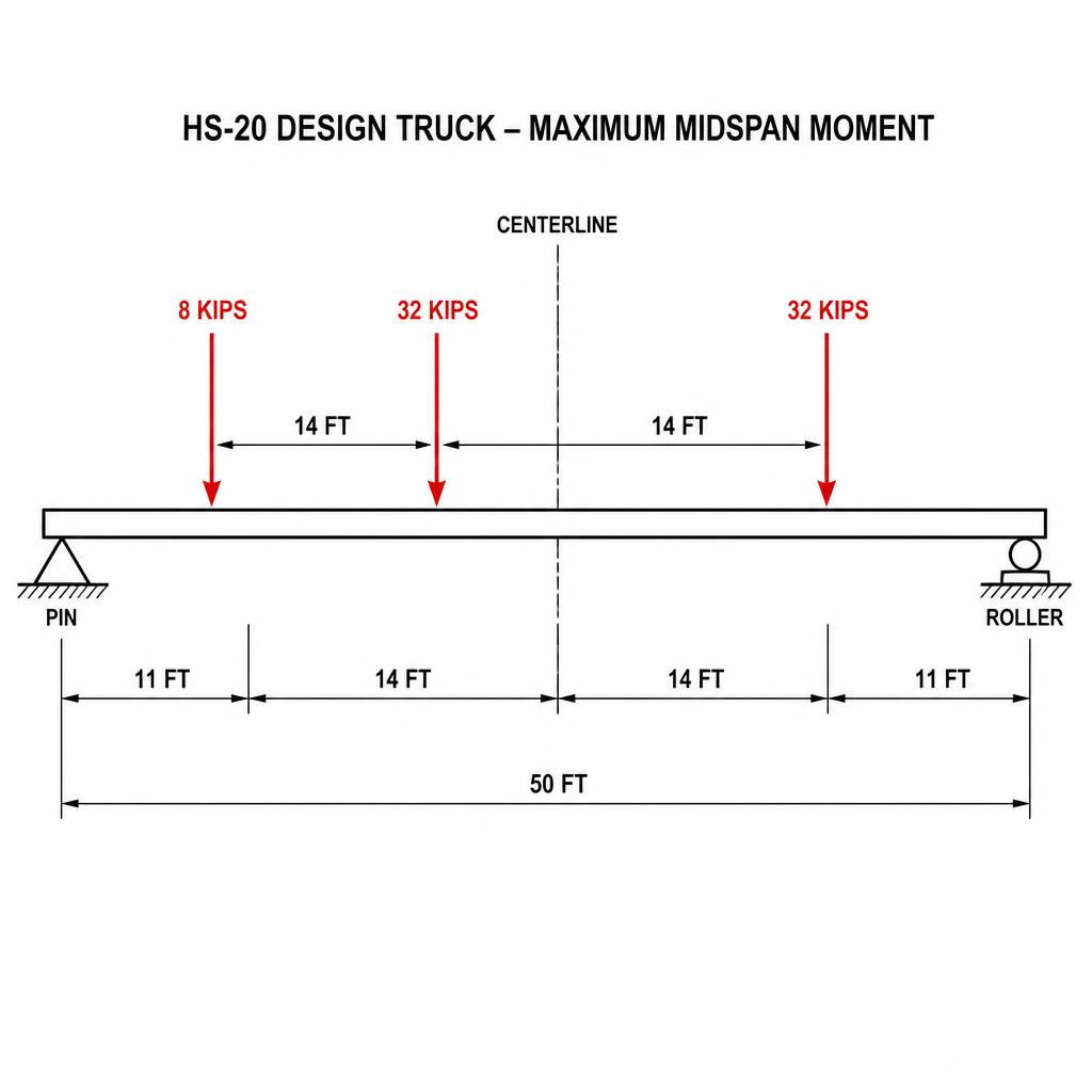
3 axles: 8 kip + 32 kip + 32 kip. First spacing 14 ft. Variable rear spacing 14–30 ft — vary to maximize the effect.
Design tandem
2 axles of 25 kip at 4 ft. Controls short spans and short-loaded lengths.
Design lane load
0.64 klf uniformly distributed over a 10-ft-wide strip. No IM applied to the lane load.
The governing document
All rules, factors, and combinations in this chapter derive from the AASHTO LRFD Bridge Design Specifications, 10th Edition (2024). Every equation cited with an AASHTO reference is verified against this edition. Older editions used different HL-93 load factors and IM values — always check the edition printed on the cover before using published examples.
AASHTO LRFD Reference
3.3 — Modifiers
Dynamic allowance and multiple-presence
The static HL-93 forces are amplified for dynamic vehicle–bridge interaction (bouncing, pothole strike, joint impact) using the dynamic load allowance IM, and reduced for the low likelihood that all traffic lanes are simultaneously loaded to maximum using the multiple-presence factor m.
Formula
Applied to truck / tandem only
| Component | IM | Applies to |
|---|---|---|
| Deck joints — all limit states | 75% | Deck panel at expansion joint |
| Fatigue and fracture | 15% | Truck only, fatigue limit state |
| All other components | 33% | Truck / tandem, Strength & Service |
| Number of loaded lanes | Multiple-presence factor m | Rationale |
|---|---|---|
| 1 | 1.20 | Single lane loaded — one heavy truck likely to appear in its worst position |
| 2 | 1.00 | Base case; HL-93 was calibrated at m = 1.00 |
| 3 | 0.85 | Low probability all three lanes simultaneously at maximum |
| ≥4 | 0.65 | Very low probability all lanes simultaneously at maximum |
A common student error
Multiple-presence m is not applied when fatigue is under consideration, and it is not applied when the empirical live-load distribution factor is used — those DFs already include m internally. Applying m twice is an easy way to overestimate demand by 20% on a single-lane bridge.
3.4 — Combinations
Which factors, in which state?
AASHTO LRFD requires the engineer to check every relevant limit state — a boundary between acceptable and unacceptable performance. Each limit state is expressed as a linear combination of factored loads and compared to the corresponding factored resistance:
Total factored demand (left) must not exceed factored resistance (right).
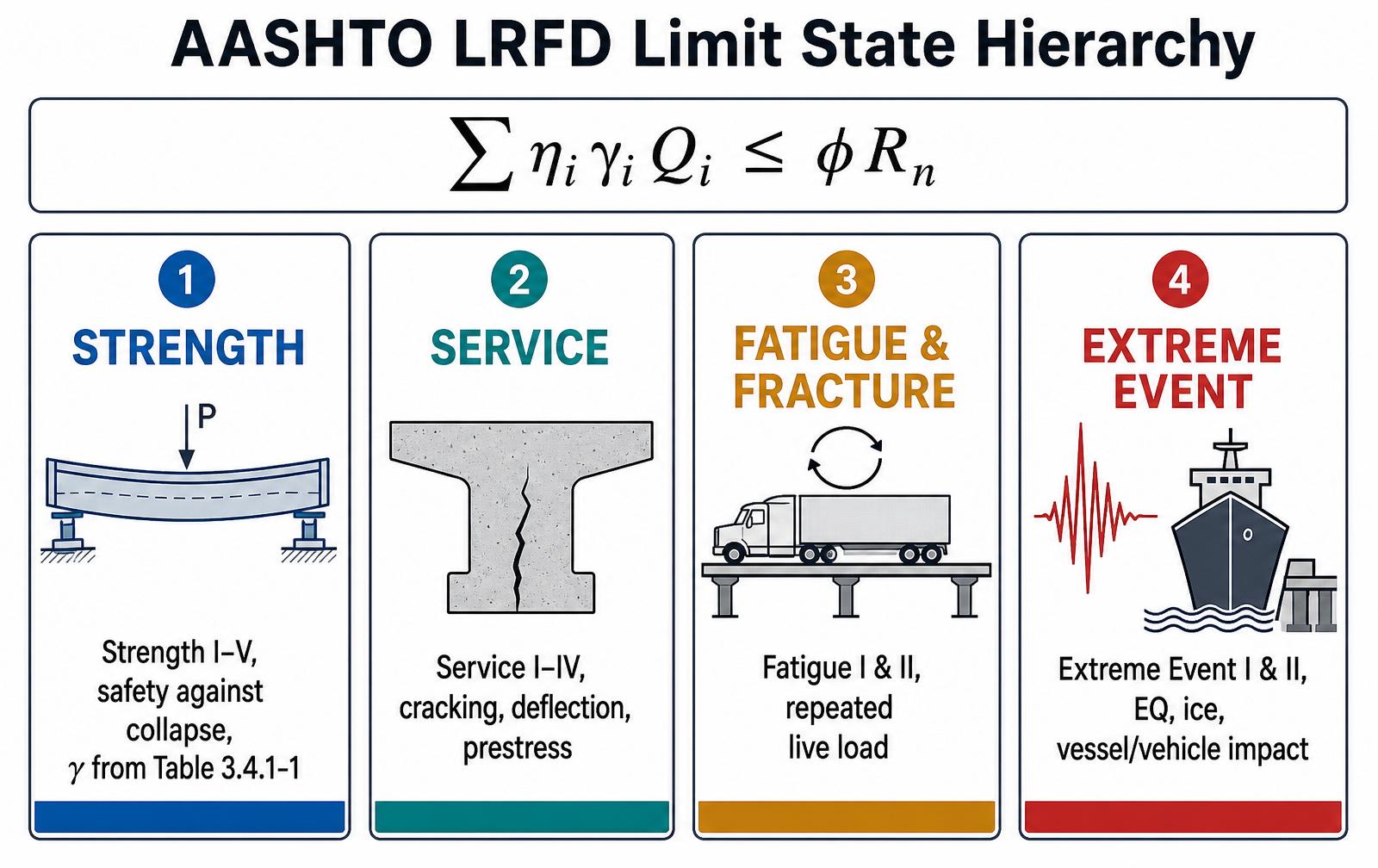
The following table lists the most commonly used highway load factors from the AASHTO LRFD 10th Edition. Values shown are maximum load factors; minimum values (used when a load is favorable to the response) are noted where required.
| Combo | DC | DW | LL + IM | BR | WS | TU | Purpose |
|---|---|---|---|---|---|---|---|
| Strength I | 1.25 | 1.50 | 1.75 | 1.75 | — | 0.50 | Normal use, no wind |
| Strength II | 1.25 | 1.50 | 1.35 | 1.35 | — | 0.50 | Permit vehicles |
| Strength III | 1.25 | 1.50 | — | — | 1.00 | 0.50 | Bridge with wind > 55 mph, no live load |
| Strength V | 1.25 | 1.50 | 1.35 | 1.35 | 1.00 | 0.50 | Normal use with wind |
| Service I | 1.00 | 1.00 | 1.00 | 1.00 | 0.30 | 1.00 / 1.20 | Deflection, prestress compressive |
| Service II | 1.00 | 1.00 | 1.30 | 1.00 | — | 1.00 / 1.20 | Steel yield / bolt slip |
| Service III | 1.00 | 1.00 | 0.80 | — | — | 1.00 / 1.20 | PC tensile stresses |
| Fatigue I | — | — | 1.75 | — | — | — | Infinite-life fatigue |
| Fatigue II | — | — | 0.80 | — | — | — | Finite-life fatigue |
| Ext. Event I | 1.25 | 1.50 | 0.50 | 0.50 | — | — | Seismic |
| Ext. Event II | 1.25 | 1.50 | 0.50 | 0.50 | — | — | Ice, collision, vessel impact |
Values are max factors; Service I TU shows force-effect / deformation split. Consult the current AASHTO LRFD table for the complete matrix including wave, ice, temperature-gradient, and vehicle-collision entries.
3.5 — Interactive activity
Position the HL-93 truck on an influence line
Manipulate the truck below to find the maximum moment and shear at any section on a 120-ft simply supported span. This is the same core operation the software performs when computing envelopes, and it should be routine before you trust any commercial output.
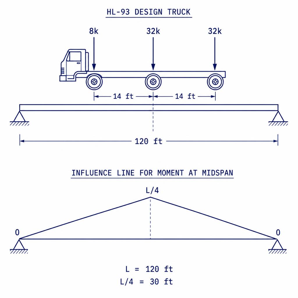
Drag the truck along the span and reposition the analysis section. AASHTO LRFD §3.6.1.2 — Design Vehicular Live Load
Moment at x = 60.0 ft
kip-ft (unfactored, per lane, IM not applied)
Shear at x = 60.0 ft
kip (unfactored, per lane, IM not applied)
How to use this
- Set the section (x/L) where you want the maximum effect.
- Slide the truck until the heaviest axles align under the peak ordinate.
- For shear at the end, sweep the truck toward the support; the lane load ordinate is largest just past the cut.
- Change the variable spacing (14 ft governs for most spans < 100 ft; 30 ft can govern for shear at far support on long spans).
3.6 — Calculator
HL-93 force-effect calculator
Use the interactive calculator to explore how span length, IM, number of loaded lanes, and multiple-presence factor combine into per-lane envelopes. The report at the bottom is exportable for your notes.
Computes the maximum midspan moment and end shear from the HL-93 envelope. AASHTO LRFD §3.6.1.2 / §3.6.2
Max midspan moment
kip-ft per design lane × factors
M = m · n · [(1+IM)·max(M_truck, M_tandem) + M_lane]
- M_truck (per lane)
- 1883.0 kip-ft
- M_tandem (per lane)
- 1450.3 kip-ft
- M_lane (per lane)
- 1152.0 kip-ft
- Governs
- Design truck
Max end shear
kip per design lane × factors
V = m · n · [(1+IM)·max(V_truck, V_tandem) + V_lane]
- V_truck (per lane)
- 60.80 kip
- V_tandem (per lane)
- 49.17 kip
- V_lane (per lane)
- 38.40 kip
- Governs
- Design truck
- w
- design lane load intensity [klf]
- L
- simply supported span length [ft]
- IM
- dynamic load allowance (33% typ.) [-]
- m
- multiple-presence factor [-]
Verification
Order-of-magnitude check: for L = 120 ft, the HL-93 envelope (per lane, per AASHTO tables) gives M ≈ 2,090 kip-ft (unfactored, no IM, no m). With IM = 1.33 and m = 1.00 the moment should approach ≈ 2,780 kip-ft plus lane contribution. Compare to the value returned above.
What can go wrong
This calculator idealizes a simply supported span. For continuous spans, use influence surfaces and apply the truck + lane combination for positive moment and two trucks (min. 50 ft between axles) × 0.90 + two lanes for negative moment AASHTO LRFD §3.6.1.3.1. Consult refined analysis for skew and curved bridges.
Governing vehicle: Design truck for moment (1883 vs 1450 k-ft truck/tandem), Design truck for shear. Design MLL+IM = 3656 k-ft, design VLL+IM = 119.3 kip on a 120 ft span.
The calculator returns per-lane envelopes; you still need distribution factors (Chapter 4) to obtain girder-line demands.
3.7 — Worked example
Worked examples: from AASHTO tables to a designed girder line
Section 3.7 works two examples end-to-end. Example 1 is the classical AASHTO reinforced-concrete T-beam bridge — a short simple span where every step (section properties, HL-93 truck / tandem / lane loads, distribution factors, dead loads, Strength I combinations) can be done by hand. Example 2 scales the same workflow up to a three-span continuous steel plate-girder bridge used in Mid-Atlantic practice.
3.7 — Example 1
Reinforced-concrete T-beam bridge (L = 50 ft simple span)
Problem statement. A bridge is to be designed with a span length of L = 50 ft. The superstructure consists of five T-beams spaced at S = 10 ft with a cast-in-place reinforced-concrete deck slab of ts = 9 in. The overall width is 48 ft and the clear (roadway) width is 44 ft 6 in. Design the superstructure of the T-beam bridge using the specifications below. The three limit states considered are Strength I, Fatigue II, and Service I.
| Symbol | Description | Value |
|---|---|---|
| C&P | Curb + parapet cross-section area | 3.37 ft² |
| Ec | Modulus of elasticity of concrete | 4 × 10³ ksi |
| f′c | Specified compressive strength of concrete | 4.5 ksi |
| fy | Yield strength of epoxy-coated rebar | 60 ksi |
| wc | Unit weight of concrete | 0.15 kcf |
| wFWS | Future wearing surface | 0.03 ksf |
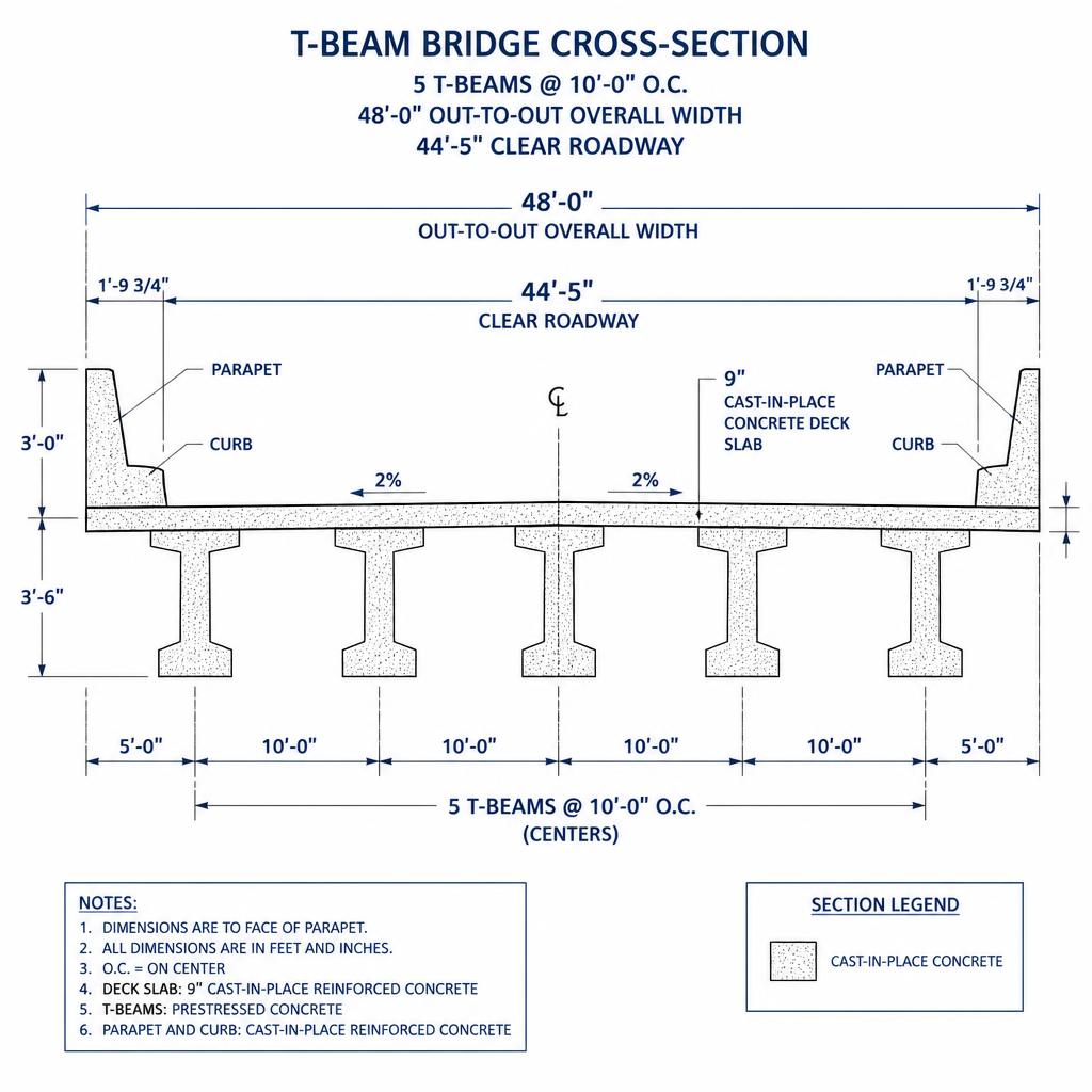
Roadmap for this example
Strength I factored load Q
The Strength I combination weights dead loads (DC, DW) and live loads (TL = truck, LN = lane) by AASHTO Tables 3.4.1-1 and 3.4.1-2. This is the equation every subsequent step feeds:
Choose deck thickness and stem width
What we are doing: pick minimum trial dimensions that (a) satisfy AASHTO minimums for a T-beam serving as its own deck and (b) leave room for two layers of #11 bars in the stem.
- Minimum deck thickness for a T-beam deck slab ≥ 7 in AASHTO LRFD §5.14.1.5.1a, §9.7.1.1. Try ts = 9 in.
- Minimum web thickness = 8 in AASHTO LRFD Com. §5.14.1.5.1c.
- Concrete cover for main epoxy-coated bars ≥ 1 in; use 1.5 in for main + stirrups AASHTO LRFD Tbl. 5.12.3-1.
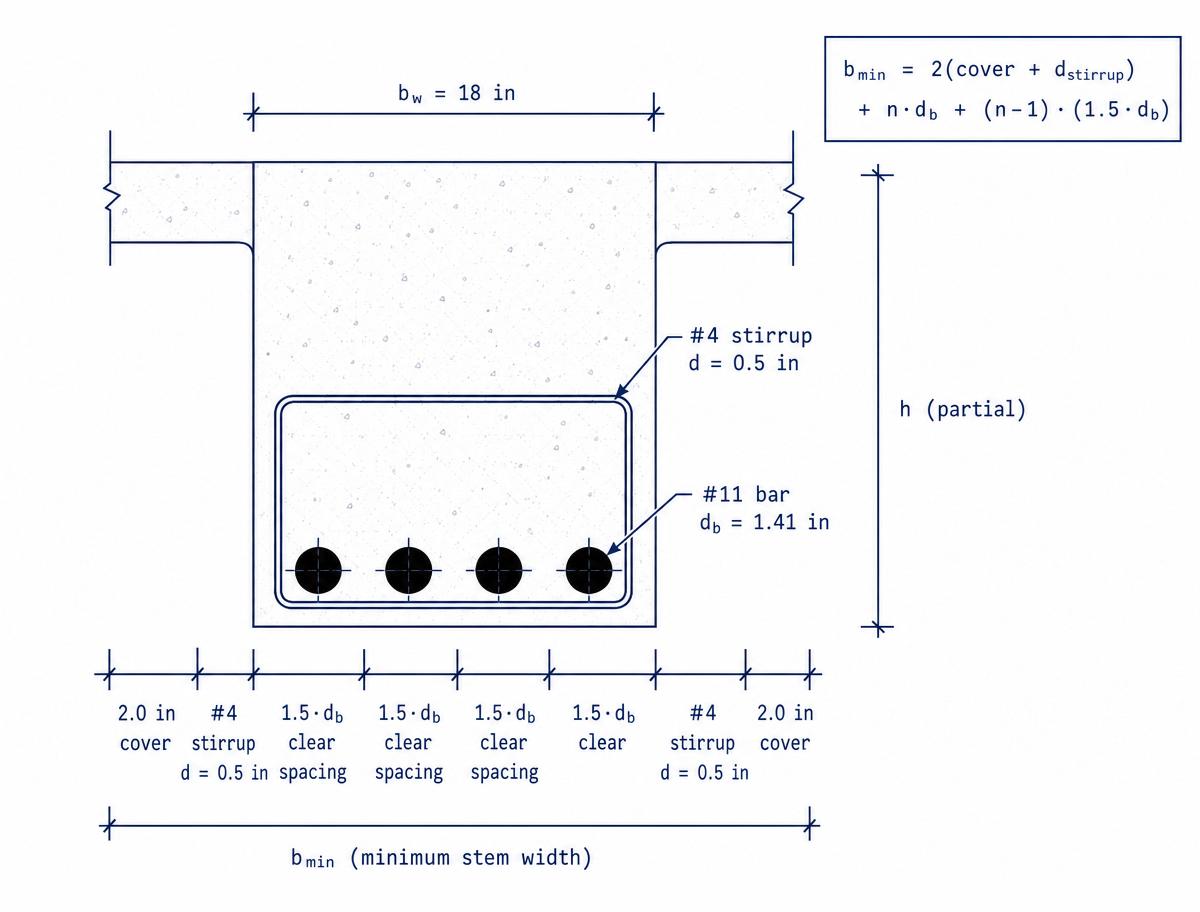
Minimum stem width for four #11 bars in a single row with #4 stirrups and 2.0 in clear cover. Write the formula first, then substitute:
Formula
Substitute
cover = 2.0 in, d_stirrup (#4) = 0.5 in, n = 4, d_b (#11) = 1.41 in
Result
Round up: try bw = 18 in.
Beam depth (including deck)
What we are doing: AASHTO Table 2.5.2.6.3-1 gives a minimum overall depth ratio for reinforced-concrete T-beams to control deflection without an explicit deflection check.
Try h = 44 in (stem = 35 in + deck = 9 in).
Effective flange width
Why: shear-lag makes only a portion of the wide slab effective in compression at midspan. AASHTO gives simple limits AASHTO LRFD §4.6.2.6.1.
- Interior beam: bi = S = 10 ft · 12 = 120 in
- Exterior beam: be = ½·S + overhang = ½·(10 ft · 12) + (4 ft · 12) = 108 in
Interior T-beam section properties
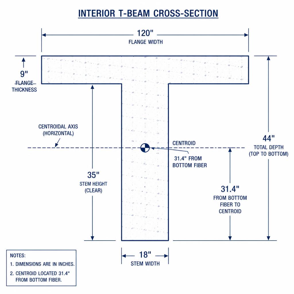
What we are doing: the moment demand from Strength I acts about the composite T-beam's centroid; we need ȳ, Ig, and S to size reinforcement in later chapters.
Area
Centroid from bottom
Parallel-axis theorem numerator ÷ total area
Moment of inertia about the centroid
Section modulus
Number of design lanes
What we are doing: the number of loaded lanes controls the multiple-presence factor and how many trucks we must place side-by-side.
Truck and tandem live-load effects per lane
What we are doing: maximum simple-span moment under HS-20 occurs with the center 32-kip axle at midspan (Barré's theorem gives the same result within rounding for the 14-14 spacing). We take moments about the right support to get the reaction, then compute midspan moment. Simple-beam influence-line ordinates at the load positions give shears.
Formula (midspan moment from statics). Sum axle contributions using the influence-line ordinate at midspan, ηi = min(xi, L − xi)·½:
Formula
Substitute HS-20 truck
Center 32-k axle at midspan; arms a₁ = 5.5 ft (8-k), a₂ = 19.5 ft (center 32-k), a₃ = 33.5 ft (rear 32-k)
Substitute HS-20 tandem
Two 25-k axles at 4 ft, centered at midspan
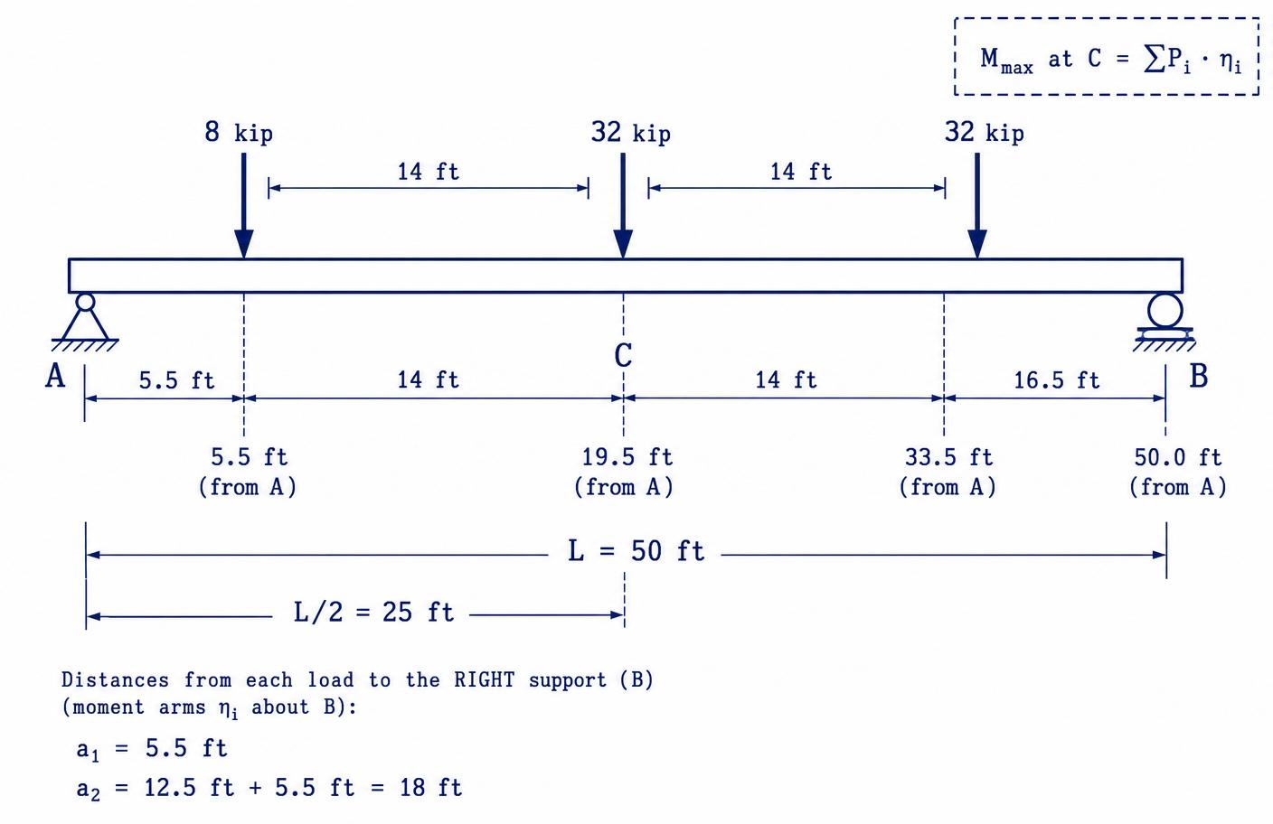
Formula (shear at left support). Using the shear influence line ηV(x) = (L − x)/L for loads to the right of the support:
Formula
Substitute truck at support
Lead 32-k axle at A, so η values are 1.00, 0.72, 0.44
Substitute tandem straddling the support
η = 1.00, 0.92
Lane load effects per lane
What we are doing: AASHTO's 0.64 klf design lane load carries no IM; use standard uniformly-loaded simple-beam formulas.
Distribution factors for moment (DFM)
Why: the truck sits on one lane, but its load spreads to several girders. AASHTO Table 4.6.2.2.2b-1 gives closed-form DFMs for cast-in-place T-beam decks (deck type "e"). Applicability checks: 3.5 ≤ S = 10 ≤ 16 ft, 4.5 ≤ ts = 9 ≤ 12 in, 20 ≤ L = 50 ≤ 240 ft, Nb = 5 ≥ 4. ✓
Longitudinal stiffness parameter (n = 1 for monolithic T-beam):
Longitudinal stiffness parameter
Interior beam — one lane loaded
Interior beam — two or more lanes loaded
Governs interior
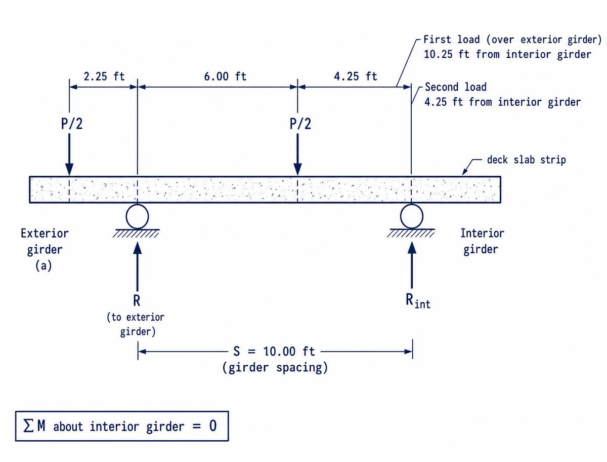
Exterior beam — one lane loaded (lever rule). Treat the deck strip as simply supported between the exterior girder and the first interior girder. Multiple-presence m = 1.20 applies with the lever rule.
Formula. Sum moments about the interior girder support (ΣM = 0), then apply m:
Formula
Substitute
S = 10 ft, a₁ = 10.25 ft, a₂ = 4.25 ft, m = 1.20
Governs exterior
Exterior beam — two or more lanes (e-factor on interior DF):
Distributed live-load moments per beam
What we are doing: multiply the per-lane truck/tandem/lane moment by the governing DFM. Apply IM = 33% to truck/tandem onlyAASHTO LRFD Tbl. 3.6.2.1-1.
| Beam | MTL (truck) [kip-ft] | MLN (lane) [kip-ft] |
|---|---|---|
| Interior (DFM = 0.859) | 620·0.859·1.33 = 708.33 | 200·0.859 = 171.8 |
| Exterior (DFM = 0.87) | 620·0.87·1.33 = 717.40 | 200·0.87 = 174.0 |
Distribution factors for shear (DFV) and shears per beam
What we are doing: shear DFs come from a different AASHTO table (AASHTO LRFD §4.6.2.2.3). Shear DFs do not include a Kgterm — the response is more local.
Governs interior
Governs exterior, lever
| Beam | VTL [kips] | VLN [kips] |
|---|---|---|
| Interior (DFV = 0.95) | 58.6·0.95·1.33 = 74.04 | 16·0.95 = 15.2 |
| Exterior (DFV = 0.87) | 58.6·0.87·1.33 = 67.80 | 16·0.87 = 13.92 |
Dead-load force effects
What we are doing: the T-beam stem, deck flange, and curb-and-parapet are part of the section → DC. The 2-in future overlay is not → DW. Distribute both as uniform loads and apply wL/2 and wL²/8.
Interior beam (self-weight includes full effective flange):
Exterior beam — deck slab + FWS reactions come from statics on the overhang. Deck-slab pressure: ws = (9/12)·0.15 = 0.113 ksf; FWS: 0.03 ksf; total 0.143 ksf. Taking moments about the first interior support gives RA = 1.31 klf (deck + FWS combined). Splitting proportionally:
From overhang statics on 0.51 klf line load
Assemble Strength I demands and identify controls
What we are doing: plug the unfactored effects into Q = 1.25·DC + 1.50·DW + 1.75·(TL + LN) and compare interior vs. exterior girders to identify the governing case that Chapter 8 (flexure) and Chapter 6 (shear) must resist.
| Effect | Interior beam | Exterior beam |
|---|---|---|
| MDC | 618.75 | 756.3 |
| MDW | 93.75 | 84.4 |
| MTL | 708.33 | 717.4 |
| MLN | 171.8 | 174.0 |
| VDC | 49.5 | 60.5 |
| VDW | 7.5 | 6.75 |
| VTL | 74.04 | 67.8 |
| VLN | 15.2 | 13.92 |
All moments in kip-ft; shears in kips.
Controls shear
Controls moment
Governing demands hand off to design
3.7 — Example 2
Three-span Maryland highway bridge (90-120-90 ft): loads & combinations
This example uses a representative Mid-Atlantic bridge configured to reflect typical MDOT SHA practice. It follows the same 13-step calculation format used in Example 1.
Interpret the problem
Determine the unfactored and factored dead-load, live-load, and secondary force effects for an interior steel plate-girder line in the 120-ft center span of a three-span continuous highway bridge. Result feeds the Strength I, Service II, and Fatigue I combinations required for Chapter 8 girder design.
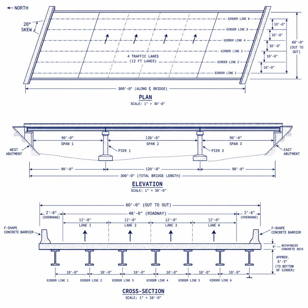
Draw the structural system
Declare known information
| Structure | 3 continuous steel plate girders, spans 90-120-90 ft |
| Deck width | 60 ft out-to-out; 48 ft roadway (4 lanes @ 12 ft) |
| Girders | 6 girder lines, spaced S = 10 ft, exterior overhang = 2.5 ft |
| Skew | 20° |
| Deck slab | 9-in cast-in-place reinforced concrete, γc = 150 pcf |
| Barrier | 36-in F-shape concrete, 0.42 klf per barrier |
| Future wearing surface | 2-in bituminous overlay, 0.025 ksf per MDOT SHA |
| Utilities | 3-in ductile-iron waterline on fascia, 0.08 klf on one exterior girder |
| Steel girder self-weight | 0.35 klf (est., interior girder) |
| Stay-in-place forms | 0.015 ksf between girders |
| Live load | HL-93 per AASHTO LRFD §3.6.1.2, IM = 33% (Strength/Service) |
Declare required results
- Unfactored DC and DW moments at the 0.4·L point of the 120-ft center span (interior girder).
- Unfactored HL-93 LL + IM moment envelope in the center span (per lane).
- Distribution factor for one design lane loaded (interior girder, moment).
- Strength I, Service II, and Fatigue I demand moments at the 0.4·L point.
Identify governing provisions
- AASHTO LRFD §3.3.2— load notation
- AASHTO LRFD §3.5.1— permanent loads DC/DW
- AASHTO LRFD §3.6.1.2— HL-93
- AASHTO LRFD §3.6.1.3.1— continuous-span rules
- AASHTO LRFD §3.6.2.1— IM = 33% for Strength/Service, 15% for Fatigue
- AASHTO LRFD §4.6.2.2.2b— live-load distribution factor for moment
- AASHTO LRFD §3.4.1 Table 3.4.1-1— load combinations
State assumptions
- Composite behavior in positive-moment regions after deck cures.
- Beam-line analysis is adequate for preliminary demand estimation (§4.6.2.1).
- Skew ≤ 20° — no distribution-factor skew correction required for interior girder moment (§4.6.2.2.2e-Table 1).
- Utilities lumped on one exterior girder; other exterior carries none. Interior girders unaffected.
- Stay-in-place forms treated as DC (non-composite steel-only stage) per MDOT SHA.
Write the governing equations
Interior girder, per unit length
Evenly distributed, MDOT SHA
Interior girder DW
Stay-in-place forms, DC non-composite
Self-weight
Substitute values (dead loads)
| w_deck | (150 pcf) · (9/12 ft) · (10 ft) = 1.125 klf |
| w_barrier per girder | (2 × 0.42) / 6 = 0.140 klf |
| w_FWS | 0.025 ksf · 10 ft = 0.250 klf |
| w_SIP | 0.015 ksf · 10 ft = 0.150 klf |
| w_girder | 0.35 klf |
| Σ DC (interior) | w_deck + w_barrier + w_SIP + w_girder = 1.125 + 0.140 + 0.150 + 0.35 = 1.765 klf |
| DW | 0.250 klf |
Calculate dead-load moments at 0.4·L (center span)
For a continuous three-span beam with uniform load and span ratio 90:120:90, the moment at the 0.4·L point in the center span from a uniform load w on all spans is well approximated (from three-moment analysis) by:
Interior span, all-spans loaded
| M_DC | 0.083 · 1.765 · (120)² = 0.083 · 1.765 · 14,400 ≈ 2,110 kip-ft |
| M_DW | 0.083 · 0.250 · (120)² ≈ 299 kip-ft |
What can go wrong
Compute HL-93 LL + IM in the center span (per lane)
For positive moment in the center span, place one design truck in the center span with lane load also in the center span (§3.6.1.3.1). A direct calculation using the 120-ft simply supported equivalent (upper bound; refined continuous analysis is slightly lower) gives:
| Truck M (unfactored, simply supported) | ≈ 1,861 kip-ft |
| Tandem M (unfactored, simply supported) | ≈ 1,462 kip-ft |
| Lane M = 0.64 · 120² / 8 | = 1,152 kip-ft |
| Envelope per lane (with IM = 33%) | 1.33 · 1861 + 1152 = 3,627 kip-ft |
Design check
Distribution factor for interior girder (moment)
Compute Kg (longitudinal stiffness parameter) from the composite section. For this example, using representative non-composite steel-girder properties (Isteel = 47,000 in⁴, A = 68 in², eg = 34 in from girder N.A. to deck centroid, deck n = 8):
Formula
Substitute
| (S/14)^0.4 | (10/14)^0.4 = 0.878 |
| (S/L)^0.3 | (10/120)^0.3 = 0.469 |
| [Kg / (12·L·ts³)]^0.1 | [1.0e6 / (12·120·9³)]^0.1 = [1.0e6 / 104,976]^0.1 = 9.526^0.1 = 1.253 |
| DF (one lane) | 0.06 + 0.878 · 0.469 · 1.253 = 0.06 + 0.516 = 0.576 |
For two design lanes loaded, DF = 0.075 + (S/9.5)^0.6 · (S/L)^0.2 · [Kg/(12·L·ts³)]^0.1 ≈ 0.755. Two-lane DF typically governs interior girders — use the larger.
Assemble Strength I, Service II, Fatigue I demands (interior girder, 0.4·L)
| Combination | Expression | Value (kip-ft) |
|---|---|---|
| Strength I | 1.25·MDC + 1.50·MDW + 1.75·MLL+IM | 1.25·2110 + 1.50·299 + 1.75·2738 = 2637 + 448 + 4791 = 7,876 |
| Service II (steel) | 1.00·MDC + 1.00·MDW + 1.30·MLL+IM | 2110 + 299 + 1.30·2738 = 2110 + 299 + 3559 = 5,968 |
| Fatigue I (LL only) | 1.75 · (1.15 · truck at 30-ft rear spacing, DF for fatigue, per lane, m=1.0) | ≈ 1,470 (see Chapter 17 for full derivation) |
Independent verification and final summary
- Order-of-magnitude: A 120-ft continuous steel-girder span at typical demand ratios has M_Str-I ~ 6,500 – 9,000 kip-ft per interior girder — our 7,876 kip-ft sits mid-range. ✓
- Unit check: All moments in kip-ft; distribution factor dimensionless. ✓
- Envelope check: Strength I > Service II — as expected for a 1.75 vs. 1.30 LL factor combined with the same DC/DW. ✓
- Sensitivity: Increasing S from 10 to 11 ft raises DF to ≈ 0.82 and M_LL+IM (girder) to ≈ 2,980 kip-ft, raising Strength I demand to ≈ 8,300 kip-ft (+5.4%). Girder spacing is a strong lever.
Final design summary — interior girder, 0.4·L, 120-ft center span
- MDC
- 2,110 kip-ft
- MDW
- 299 kip-ft
- MLL+IM (per lane env.)
- 3,627 kip-ft
- DF (2-lane)
- 0.755
- MLL+IM (girder)
- 2,738 kip-ft
- Strength I
- 7,876 kip-ft
- Service II
- 5,968 kip-ft
- Fatigue I (LL only)
- ≈ 1,470 kip-ft
Design status
3.8 — Design challenge
T-beam bridge — full load & section-property workup
Apply everything from Chapter 3 (and the pre-lecture on section properties) to the simply-supported reinforced-concrete T-beam bridge shown below. Produce a complete hand-calculation package and upload it at the bottom of this section.
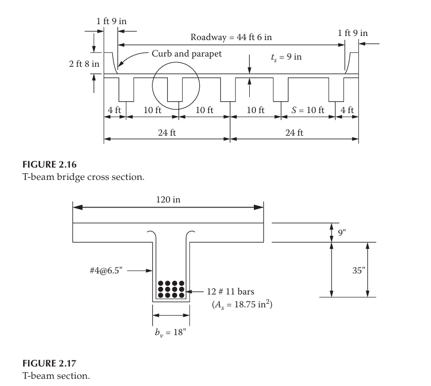
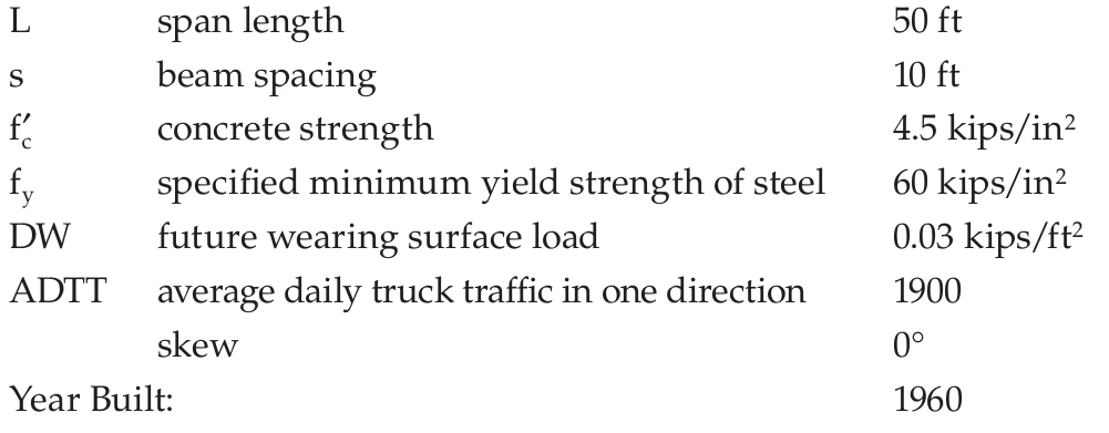
Deliverables — compute and report for BOTH an interior and an exterior girder
- Section properties — for both the non-composite stem (bare RC T-beam before deck-slab hardens is not relevant here since this is cast-monolithic RC; still report the stem-only section as reference) and the composite T-section with effective flange width beff per AASHTO 4.6.2.6:
- Positive-moment region (midspan): untransformed composite section — full deck in compression. Report beff, neutral-axis depth yb, gross moment of inertia Ig, and section moduli Stop and Sbot.
- Negative-moment region: since the bridge is simply supported, there is no continuous negative-moment region. If instead the two 50-ft spans were made continuous, deck concrete cracks — the effective section is the stem plus the longitudinal deck reinforcement inside beff. Report the cracked-transformed Icr and ycr for that hypothetical continuous case (state your assumed As,deck).
- For steel-composite thinking (short- vs. long-term), state the modular ratio n = Es/Ec and 3n for long-term (creep), and briefly explain why the RC T-beam here uses a single n (all concrete).
- Permanent loads — compute per linear foot of one girder:
- DC1 — self-weight of the girder stem and the tributary deck slab (both cast monolithically, γc = 0.150 kcf). Show the tributary width you used for interior vs. exterior girders.
- DC2 — barriers/parapets (γc·A_parapet, 2 ft 8 in tall). Distribute equally to all girders per AASHTO 4.6.2.2.1 and comment on the exterior-girder exception.
- DW — future wearing surface (0.030 ksf) over the 44 ft 6 in roadway, distributed to the appropriate girders.
- SIP formwork and steel cross-frames — state whether they apply here (cast-in-place RC deck, no steel diaphragms) and justify.
Note: live-load distribution factors, per-lane HL-93 moment/shear envelopes, and per-girder MLL+IM / VLL+IM are analysisoutputs and have been migrated to the Chapter 4 design challenge (§4.7). Complete the Ch 3 items here — section properties and permanent loads — and use them as inputs to the Ch 4 challenge.
What to hand in
Submit your design challenge
Chapter 3 challenge — T-beam bridge: section properties, DC1, DC2, DW, distribution factors, live-load M & V
You must be signed in to upload a submission.
Sign in →3.9 — Graded quiz
Chapter 3 assessment (20 questions)
Twenty questions covering load categories, HL-93, IM, m, combinations, influence-line placement, and the worked example. Your attempt is recorded to your student progress.
Start Chapter 3 quiz →Chapter summary
Key takeaways
- HL-93 = (design truck OR tandem) + design lane load. IM applies only to the truck/tandem.
- Multiple-presence m = 1.20, 1.00, 0.85, 0.65 for 1, 2, 3, ≥4 loaded lanes.
- Strength I governs most normal traffic; Strength II governs permit vehicles (MDOT SHA).
- Negative moment at interior supports uses the two-truck × 0.90 rule.
- Always identify governing combination BEFORE selecting member sizes.
Section 1
Concept Demonstrations
Instructor-led walkthroughs of core ideas. Read these first — every worked example that follows builds on them.
Demo 1
Convert a deck geometry + unit weight into a distributed DC load carried by each girder.
An 8-in normal-weight concrete deck spans between girders spaced at S = 8 ft. Using γc = 0.150 kcf (0.145 kcf plain + 0.005 kcf allowance for reinforcement per AASHTO Table 3.5.1-1):
wdeck = γc · t · S = 0.150 · (8/12) · 8 = 0.800 klf per interior girder.
This is the DC1 contribution (deck acting on the non-composite girder). Add a barrier of 0.320 klf split equally to the two fascia girders, and a haunch of 0.010 klf. Note we did not apply a load factor — DC and DW are computed as unfactored demands here; γDC = 1.25 (Strength I max) is applied at the combination step.
Demo 2
The 32-kip axle drives shear near supports; the 32-32 pair drives midspan moment.
Place the HL-93 truck (8-32-32 kip, first spacing 14 ft, rear variable 14–30 ft) on a simple span. For maximum shear at the left support, the heaviest axle sits directly over the support; the influence-line ordinate is 1.0.
For maximum moment at midspan, position the truck so the load's resultant and the closest axle straddle midspan by equal amounts (Barré's theorem). On most simple spans of 40–90 ft, the two 32-kip axles at 14-ft spacing govern; on very short spans the design tandem (2 × 25 kip at 4 ft) usually controls instead.
Demo 3
IM amplifies the truck/tandem only. m modifies the sum of live-load effects across loaded lanes.
Compute the raw static effect of truck (or tandem) and lane separately. Apply IM = 33% (Strength/Service) to the truck/tandem only. Combine the amplified truck with the lane load. Then, if two lanes are simultaneously loaded, multiply the two-lane result by m = 1.00; one-lane loading uses m = 1.20; three lanes m = 0.85.
LL+IM (per lane) = 1.33 · (truck or tandem) + 1.00 · (0.64 klf lane load)
IM is never applied to the lane load or to pedestrian, wind, or thermal loads.
Demo 4
Strength I dominates highway girders; Strength III/V come in only when wind is significant.
For a typical highway girder in the Mid-Atlantic, Strength I:
η · [1.25·DC + 1.50·DW + 1.75·(LL+IM) + 1.00·(WA + FR) + 0.50·TU]
controls positive and negative moment envelopes 95% of the time. Strength III (wind without LL) and Strength V (wind with LL at 55 mph reference) become relevant only for tall piers, long-span steel plate girders, or superstructures with high W/D. Extreme Event I (EQ) and Extreme Event II (CT/CV/IC) always accompany a Strength I check — never as the sole envelope.
Section 2
Fully Worked Examples
Complete AASHTO LRFD solutions with knowns, assumptions, step calculations, verification, and design commentary. Difficulty rises from basic to consulting-grade.
Worked Example 1
Problem
Step-by-Step
w = 0.150 · (8/12) · 8 = 0.800 klf
0.800 klf
W36×150 = 0.150 klf.
0.150 klf
Design Verification
Total unfactored dead load on the interior girder: 0.97 + 0.128 + 0.187 ≈ 1.29 klf. Compare against DC + DW ≈ 1.3 klf typical for this bridge type (spot check passes).
Discussion
DC and DW are separated because DW carries a larger max factor (1.50 vs 1.25). MDOT SHA also requires a minimum DW of 0.025 ksf even when no overlay is planned, to hedge against 75-year rehabilitation cycles.
Worked Example 2
Problem
Step-by-Step
M = wL²/8 = 0.64·90²/8 = 648 k·ft
648 k·ft
M = wx(L−x)/2 = 0.64·22.5·67.5/2 = 486 k·ft
486 k·ft
Design Verification
M_L/4 / M_L/2 = 486/648 = 0.75, matches parabolic UDL moment ratio (3/4). ✓
Discussion
The lane load contributes typically 30–45% of the total LL+IM moment on medium spans; the truck governs the rest.
Worked Example 3
Problem
Step-by-Step
R = 72 kip. Distance of R from lead 8-kip axle: x̄ = (32·14 + 32·28)/72 = 18.67 ft.
R = 72 k at 18.67 ft aft of lead axle
Place the middle 32-k axle at midspan + (18.67 − 14)/2 = 2.33 ft toward the lead. Then M is maximum under that axle.
Middle axle at x = 45 − 2.33 = 42.67 ft from left support
Design Verification
Combine with lane load (Ex. 2): 1788 + 648 = 2436 k·ft per lane, LL+IM. Rule-of-thumb approximate M_HL-93 ≈ 0.10·wL² using w ≈ 3 klf equivalent gives ≈ 2430 k·ft — matches within 1%. ✓
Discussion
The variable rear axle at 14 ft gives max moment; only for very long spans (L > 145 ft) does opening to 30 ft alter M appreciably.
Worked Example 4
Problem
Step-by-Step
Full 28-ft truck length fits within 30 ft. Position for max M: place 32-k axle 2.0 ft right of midspan (Barré with front pair, resultant of 8+32=40 k at 11.2 ft aft of lead).
Two axles engage; rear 32-k off span
Using R and geometry: M_truck ≈ 250 k·ft (verify via influence lines).
≈ 250 k·ft
Design Verification
Tandem > truck for L < ≈ 40 ft — matches AASHTO commentary and NCHRP 12-33 calibration curves.
Discussion
Never assume the truck always governs — for approach slabs, short overpasses, and rating of legacy short-span bridges, the tandem controls.
Worked Example 5
Problem
Step-by-Step
DF₁ = 0.06 + (S/14)^0.4 · (S/L)^0.3 · [K_g/(12·L·t_s³)]^0.1
= 0.06 + (8/14)^0.4 · (8/90)^0.3 · [6.0e6/(12·90·8³)]^0.1
= 0.06 + 0.796·0.478·1.130 = 0.06 + 0.430 = 0.490
DF₁ ≈ 0.490
DF₂ = 0.075 + (S/9.5)^0.6 · (S/L)^0.2 · [K_g/(12·L·t_s³)]^0.1
= 0.075 + (8/9.5)^0.6 · (8/90)^0.2 · 1.130
= 0.075 + 0.903·0.615·1.130 = 0.075 + 0.628 = 0.703
DF₂ ≈ 0.703 (governs)
Design Verification
Two-lane DF exceeds one-lane (as expected for S < 12 ft). Multiple-presence m is already embedded in the AASHTO empirical DF equations — don't double-count.
Discussion
The 1.20 multi-presence factor is not applied on top of Table 4.6.2.2.2b DFs, but IS applied when using the lever rule or 3-D refined analysis.
Worked Example 6
Problem
Step-by-Step
= 0.97·90²/8 = 982 k·ft
982 k·ft
= 0.128·90²/8 = 130 k·ft
130 k·ft
Design Verification
Live-load contribution 2996/4670 = 64% — typical for medium-span steel bridges. If the ratio exceeded 75%, revisit DF and cross-section.
Discussion
Service II (0.80·LL) would be used for steel-yielding overload check; Fatigue I (1.75·LL fatigue truck) for detail category checks.
Worked Example 7
Problem
Step-by-Step
Approximate each truck effect on IL: M_1truck ≈ 72 kip · (avg ordinate over 28-ft footprint). Using ordinate ≈ −0.8·|min| at each truck: M_1truck ≈ 72·(−9.6) = −691 k·ft per truck. Two trucks give −1382 k·ft.
−1382 k·ft
M_trucks = 0.90 · 1.33 · (−1382) = −1655 k·ft.
−1655 k·ft
Design Verification
Compare with single-truck result: 0.90 · 2 trucks / 1 truck ≈ 1.8× — the two-truck rule adds roughly 65–90% over single-truck negative moment on this configuration, in line with published QCONBRIDGE output.
Discussion
The 0.90 multiplier accounts for the low probability of two heavy trucks arriving with the exact 50-ft separation. Never omit it for continuous negative moment.
Worked Example 8
Problem
Step-by-Step
With 8-32-32 at 14 and 30 ft, on 90 ft, static midspan M ≈ 1155 k·ft (position resultant symmetrically). Apply IM = 15%: 1.15·1155 = 1328 k·ft.
1328 k·ft
DF_fat = DF_two / 1.20 = 0.703 / 1.20 = 0.586 (removes multi-presence built into the two-lane DF).
0.586
Design Verification
Compare ΔM against Category B constant-amplitude fatigue limit (F)_TH · S_x for the girder; if ΔF_computed < (ΔF)_TH, infinite life is achieved.
Discussion
Fatigue II (finite life) uses the single fatigue truck with γ = 0.80 and (ADTT)_SL to compute stress cycles; Fatigue I is the infinite-life screening check.
Worked Example 9
Problem
Step-by-Step
Option A: 25% of truck = 0.25·72 = 18 kip. Option B: 5% (truck + lane) = 0.05·(72+160) = 11.6 kip. Governs: 18 kip.
BR = 18 kip / lane
N_lanes = 2, m = 1.00. BR_total = 18·2·1.00 = 36 kip.
36 kip total
Design Verification
Compare to WS + WL on live load: BR frequently controls longitudinal loading on interior piers of continuous multi-span girder bridges.
Discussion
BR is applied in ALL lanes carrying traffic in the same direction. On future capacity expansion (adding a lane), re-evaluate BR — a common rehab-era oversight.
Worked Example 10
Problem
Step-by-Step
Center the 6-axle group at midspan. R_A = 220/2 = 110 kip. Sum axle contributions to M under middle axles: ≈ 2450 k·ft (computed via superposition).
M_static ≈ 2450 k·ft
M_perlane = 1.33 · 2450 = 3259; M_girder = 1.20 · 0.490 · 3259 = 1917 k·ft.
M_LL+IM = 1917 k·ft
Design Verification
Confirm permit rating factor RF = (φR_n − γ_DC·DC − γ_DW·DW) / (γ_LL·LL+IM) > 1.0. If Strength II governed and RF < 1.0, escort restrictions or overweight route reroute is required.
Discussion
Strength II is critical for load-rating and superload permitting decisions. Never assume HL-93 always envelopes — 200-kip cranes and 12-axle transformer haulers routinely control on medium spans.
Section 3
Guided Practice
Complete the missing steps. Use Hints for AASHTO article pointers and setup logic before revealing the full step. Submit at the end to send your work to your instructor.
Guided Problem 1
Interior girder of a cast-in-place T-beam bridge: web 14 in × 36 in, flange (deck) 8 in over S = 9 ft, barrier 0.310 klf each side (2 barriers ÷ 4 girders), no future overlay assumed initially, γc = 0.150 kcf.
Guided Problem 2
Simple span L = 50 ft. Determine the maximum midspan static moment from the design tandem alone, then the (LL+IM) tandem-plus-lane per-lane moment.
Guided Problem 3
Unfactored per-girder demands: DC = 1200 k·ft, DW = 250 k·ft, LL+IM = 1900 k·ft. Compute Strength I M_u.
Guided Problem 4
Exterior girder, S = 8 ft. Barrier + curb extends 2.5 ft outboard of the girder centerline. First wheel of a design truck is 2 ft from the barrier (§3.6.1.3.1: min 2 ft from curb). Compute one-lane DF by the lever rule.
Section 4
Independent Practice
Every problem randomizes its inputs. Work each step, submit for immediate feedback, request new values to practice again.
Practice 1
Practice 2
Practice 3
Practice 4
Practice 5
Practice 6
Practice 7
Practice 8
Practice 9
Practice 10
Practice 11
Practice 12
Practice 13
Practice 14
Practice 15
Section 5
Design Challenges
Multi-day projects mirroring real consulting scope. Submit a report package for review.
Project 1
Scope
Prepare Strength I, Service I, Service II, Fatigue I, and Extreme Event II load-effect envelopes at 20 tenth-points for a 90-120-90 ft, 5-girder, 42-ft-wide steel plate girder bridge. Include HL-93, MDOT SHA permit vehicle CH-64, WS, WL, TU, and CV (100-kip static impact at Pier 2).
Deliverables
- Envelope tables (M, V per limit state, 20 sections)
- Two-truck negative-moment check at Pier 2 with 50-ft-clear position sketch
- Distribution-factor calcs (interior + exterior) with lever-rule sketch
- Barrier + FWS + utility DW build-up sheet
- Signed engineering report ≤ 20 pages
Constraints
- AASHTO LRFD 10th Ed. only
- MDOT SHA superstructure manual §5.2 for permit envelope
- Report format: US letter, 11 pt serif, calc-note style
Grading Rubric
- Load categorization correctness15%
- HL-93 positioning + IM/m application20%
- Distribution-factor derivations15%
- Envelope completeness (limit states × 20 sections)25%
- Permit + extreme-event handling15%
- Report clarity and citation discipline10%
Submit your design challenge
Full load envelope for a 3-span continuous plate-girder bridge
You must be signed in to upload a submission.
Sign in →Project 2
Scope
Rate an existing 110-ft simple-span composite steel bridge (fabricated 1972, condition rating 6) for a 15-axle 350-kip transformer transport. Provide a Rating Factor by both Strength I (HL-93) and Strength II (permit) using AASHTO MBE. Recommend escort restrictions if RF < 1.00.
Deliverables
- Section property spreadsheet (composite, non-composite)
- M and V effects for HL-93 and permit vehicle
- Strength I and Strength II RF summary table
- 1-page memo to MDOT SHA Office of Bridge Development with go / no-go recommendation
Constraints
- AASHTO MBE 3rd Ed. + 2020 interims
- Existing condition inspection report attached
- Lane-closure escort is allowed
Grading Rubric
- Permit vehicle load model + IM20%
- Section property + resistance20%
- RF calculations25%
- Escort / posting recommendation logic20%
- Memo clarity15%
Submit your design challenge
Permit-load rating memo — MDOT SHA superload
You must be signed in to upload a submission.
Sign in →Section 6
FE / PE Review
Timed, randomized professional-exam-style items. Aim for 70% under the clock — clues appear after submission.
Budget: 9 min · 69 s each avg.