Bridge Analysis and Structural Modeling — Bridge Engineering & Design

Engineering story

When the model doesn't match the bridge

In 2011, a heavily instrumented rehabilitation on a curved steel plate-girder overpass in Maryland revealed that the original beam-line analysis had underestimated the interior-girder moment by nearly 18%. Two effects had been quietly ignored: torsional warping in the curved system, and a real cross-frame load path that the beam-line model could not represent. The bridge did not fail — but the load rating computed with the wrong model would have allowed a permit vehicle that was, in fact, unsafe.

Analysis is where load (Chapter 3) becomes demand on a specific member. The choice of analysis method — beam line, distribution factor, grillage, or full 3-D finite element — is not a cosmetic preference. It changes the moments and shears you design for by 10–30% for skewed, curved, or non-standard bridges. This chapter teaches you the load path, the tools to trace it, and how to check any computer answer with statics.

Chapter objectives

What you will be able to do

Learning objectives

By the end of this chapter you will be able to:

1Trace the flow of load from wheel contact patch to soil, naming every element that carries force.
2Construct influence lines for reactions, shear, and moment on simple and continuous beams by the Müller-Breslau principle.
3Position HL-93 truck, tandem, and lane loads on an influence line for maximum effect.
4Compute AASHTO approximate live-load distribution factors (DFM, DFV) for interior and exterior girders — both moment and shear.
5Apply the skew correction factors to shear and moment DFs.
6Use the lever rule and rigid-body (special) methods when the empirical formulas do not apply.
7Decide when a bridge requires refined analysis (grillage or FE) instead of beam-line + DF.
8Set up a grillage model with correct member stiffnesses and validate it against a hand check.

4.1 — Load path

From wheel to soil

Every design calculation you make assumes an implicit answer to the question: by what route does force reach the member I am designing? Get the route wrong and no amount of code compliance saves you. The load path in a slab-on-girder highway bridge has six links:

Contact patch → wearing surface. AASHTO idealizes each tire as a 10 in × 20 in rectangle (§3.6.1.2.5).
Wearing surface → deck slab. The load spreads at roughly 45° through asphalt and slab cover.
Deck slab → girders. The slab bends transversely between girders; the equivalent-strip method (§4.6.2.1) captures this.
Girders → bearings. The girder carries longitudinal moment and shear to the supports.
Bearings → substructure. Bearings transmit vertical, longitudinal (braking, thermal), and transverse (wind, centrifugal) reactions to the pier cap or abutment.
Substructure → foundation → soil. The pier column carries combined axial + moment + shear to the pile cap or spread footing, and finally to the soil.

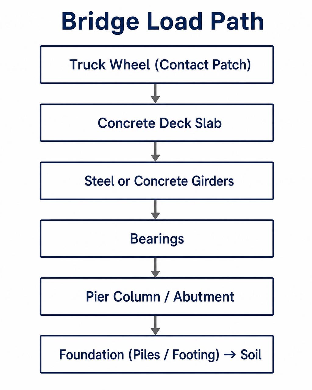
Vertical flowchart showing load path from truck wheel down through deck, girders, bearings, pier column, and drilled shafts into soil — Figure 4.1Load path from wheel contact patch to soil. Every link introduces a modeling assumption and a source of uncertainty; AASHTO's distribution factors and resistance factors are calibrated to that stack of uncertainties.

Why this ordering matters

Uncertainty accumulates as you walk down the chain. That is exactly why AASHTO uses a different resistance factor φ for each component (deck vs. girder vs. pier vs. pile) and different load factors γ for each load type — each is calibrated against the specific variability of that link in the chain.

4.2 — Influence lines

A movable-load tool

AASHTO LRFD §3.6.1.3, §4.6.2

Live loads move. To find the maximum moment or shear at a section, we need to know where to position the truck. An influence line gives, at a fixed section of interest, the value of the response (reaction, shear, moment) as a function of the position of a unit moving load. Once we have the influence line, the maximum response to a set of concentrated loads is:

(4.2-1)

Formula
$R_{max} = \sum P_{i} \cdot \eta_{i} + w \cdot A_{+}$

$R_{max}$: maximum response quantity (reaction, shear, or moment)
$P_{i}$: magnitude of the i-th concentrated wheel load [kip]
$\eta_{i}$: ordinate of the influence line at the position of load i
$w$: uniform lane load (0.64 klf for HL-93) [klf]
$A_{+}$: positive area under the influence line [ft]

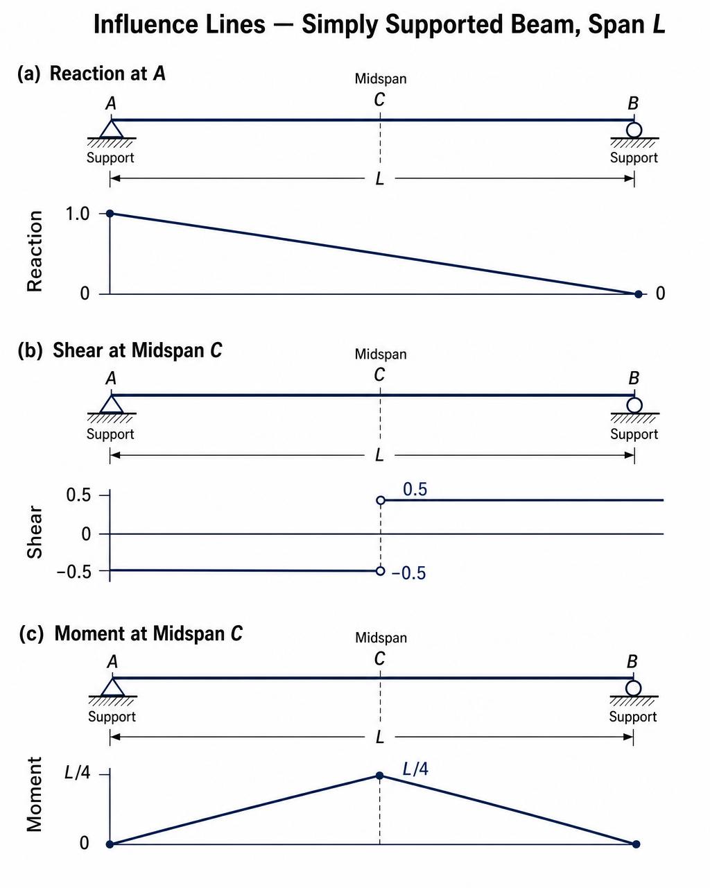
Influence lines for reaction, midspan shear, and midspan moment of a simply supported beam — Figure 4.2Influence lines for a simply supported beam of span L. (a) Reaction at A — triangle from 1 at A to 0 at B. (b) Shear at midspan C — antisymmetric, ±0.5 at midspan. (c) Moment at midspan C — triangle peaking at L/4.

4.2.1 Müller-Breslau principle

A quick physical way to construct any influence line: remove the restraint corresponding to the response you want (cut the beam for shear, insert a hinge for moment, release the support for a reaction), give a unit displacement in the positive direction of that response, and the resulting deflected shape is the influence line. This lets you sketch influence lines for continuous spans in seconds without solving the beam.

Why the shape is what it is

Reactions and moments in continuous beams give influence lines that are curved and change sign across supports. That change of sign is why continuous bridges have positive moment regions (midspan, bottom fiber in tension) and negative moment regions (over piers, top fiber in tension). Both must be enveloped when positioning live load.

4.2.2 Positioning HL-93 for maximum effect

AASHTO §3.6.1.3.1 requires the design live load to be placed such that it produces the maximum force effect on the member being checked. For a simple span:

Maximum moment — place the middle 32-kip axle of the design truck so that the resultant of the three axles and the section of interest are equidistant from midspan (the well-known "12.5 + 5.5 ft" configuration for a 60 ft span). The lane load (0.64 klf) covers the entire span.
Maximum shear at a support — place the heavy axle directly over the support; the second axle 14 ft in, the third 14–30 ft further. Lane load covers the whole span.
Maximum shear at an interior section — put the load only on the portion of the influence line that is positive (or only the negative portion for minimum shear), and let the lane load stop where the influence line changes sign.

Influence-Line Explorer — HL-93 Truck on a 120-ft Simply Supported Span

Drag the truck along the span and reposition the analysis section. AASHTO LRFD §3.6.1.2 — Design Vehicular Live Load

Truck lead-axle position (ft)30.00

Variable rear-axle spacing (ft)14.00

Section x / L0.50

Moment at x = 60.0 ft

2904.00

kip-ft (unfactored, per lane, IM not applied)

Truck axles1752.00

Design lane (0.64 klf)1152.00

Shear at x = 60.0 ft

-19.60

kip (unfactored, per lane, IM not applied)

Truck axles-29.20

Design lane (0.64 klf)9.60

How to use this

Set the section (x/L) where you want the maximum effect.
Slide the truck until the heaviest axles align under the peak ordinate.
For shear at the end, sweep the truck toward the support; the lane load ordinate is largest just past the cut.
Change the variable spacing (14 ft governs for most spans < 100 ft; 30 ft can govern for shear at far support on long spans).

4.3 — Live-load distribution factors

One girder at a time

AASHTO LRFD §4.6.2.2

A truck rolls along the deck. The transverse stiffness of the slab spreads that wheel load to every girder — but unequally. Rather than solve the coupled slab-girder system for every design, AASHTO packages the transverse distribution into a single dimensionless distribution factor (DF) that multiplies the one-lane moment/shear computed on a single beam line. This transforms a two-way problem into a one-dimensional design.

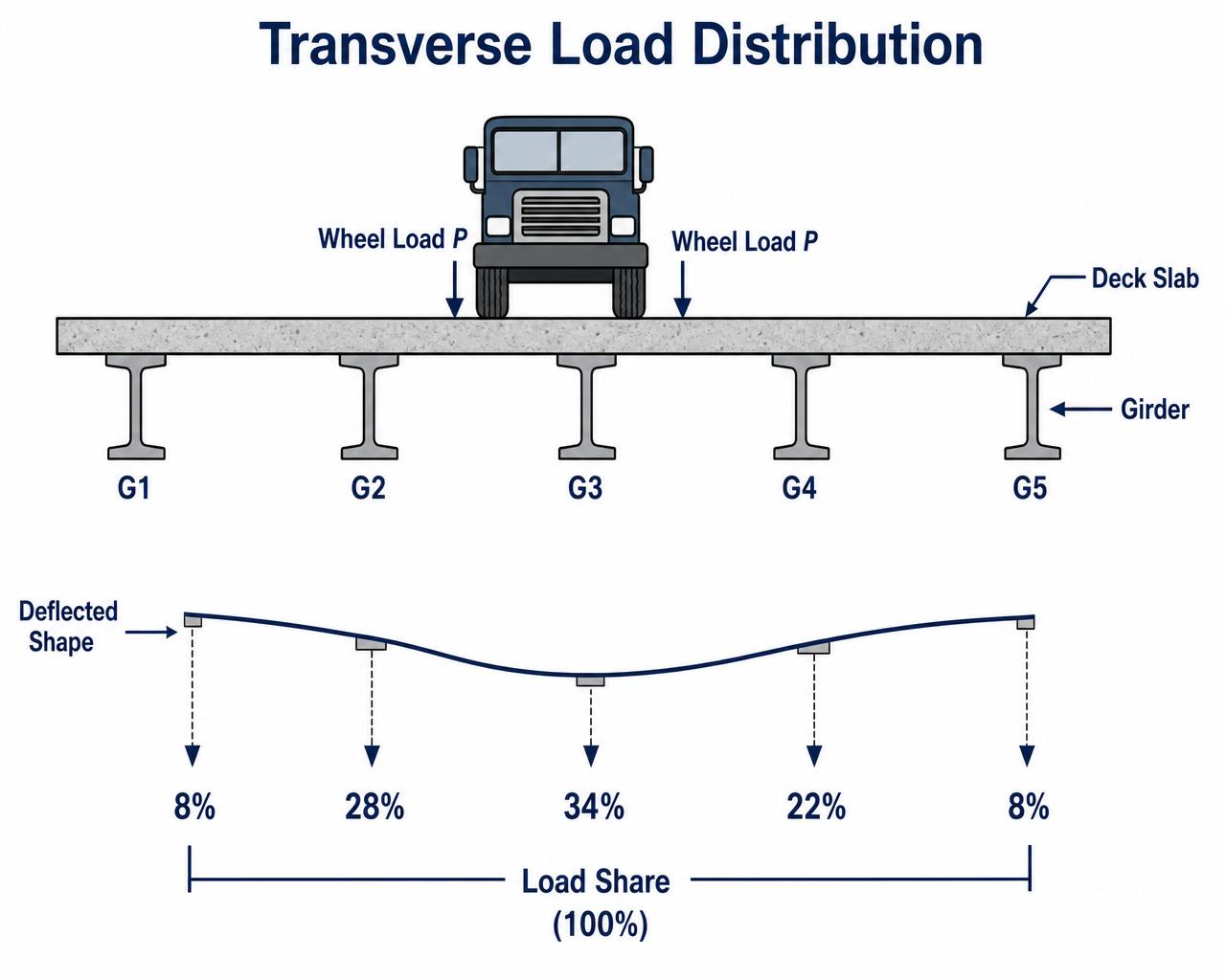
Figure 4.3Transverse distribution. The deck bends between girders and each girder picks up a share of the wheel load proportional to its transverse stiffness. AASHTO's DF equations were regressed against thousands of grillage runs to give the interior/exterior share directly.

4.3.1 Interior girder — moment (§4.6.2.2.2b)

For a slab-on-steel-girder or slab-on-prestressed-I-beam bridge with parallel girders (Table 4.6.2.2.1-1, cross-section type "a" or "k"), the empirical DF for interior girder moment is:

(AASHTO 4.6.2.2.2b-1)

One lane loaded
$DFM = 0.06 + \left(\tfrac{S}{14}\right)^{0.4} \cdot \left(\tfrac{S}{L}\right)^{0.3} \cdot \left[\tfrac{K_{g}}{12 \cdot L \cdot t_{s}^{3}}\right]^{0.1}$
Two or more lanes
$DFM = 0.075 + \left(\tfrac{S}{9.5}\right)^{0.6} \cdot \left(\tfrac{S}{L}\right)^{0.2} \cdot \left[\tfrac{K_{g}}{12 \cdot L \cdot t_{s}^{3}}\right]^{0.1}$

$S$: girder spacing [ft]
$L$: span length [ft]
$t_{s}$: deck thickness [in]
$K_{g}$: longitudinal stiffness parameter = n(I + A \cdot e_{g}^{2}) [in⁴]
$n$: modular ratio E_beam / E_deck
$I, A, e_g$: girder inertia, area, and c.g.-to-c.g. distance deck-to-girder [in⁴, in², in]

Take the larger of the two. The multiple-presence factor m is already embedded — do not multiply it in again.

AASHTO LRFD Reference

Table 4.6.2.2.1-1 — Applicability

3.5 ≤ S ≤ 16.0 ft · 4.5 ≤ t_s ≤ 12.0 in · 20 ≤ L ≤ 240 ft · N_b ≥ 4 girders · 10 000 ≤ K_g ≤ 7 000 000 in⁴. Outside these ranges the formula is not calibrated — use the lever rule or refined analysis.

4.3.2 Interior girder — shear (§4.6.2.2.3a)

(AASHTO 4.6.2.2.3a-1)

One lane
$DFV = 0.36 + \tfrac{S}{25.0}$
Two or more lanes
$DFV = 0.2 + \tfrac{S}{12} - \left(\tfrac{S}{35}\right)^{2.0}$

Shear DFs are simpler than moment DFs — shear near a support depends much less on the longitudinal stiffness parameter K_g, so it drops out of the regression.

4.3.3 Exterior girder — lever rule (§4.6.2.2.2d)

For one lane loaded on the exterior girder, AASHTO requires the lever rule: assume the deck acts as a simple beam pinned at the first interior girder, and place the wheel loads to maximize the exterior reaction.

Formula. Taking ΣM about the interior girder:

Multiply by m. For the exterior girder under the lever rule, the multiple-presence factor is not embedded — apply m = 1.20 for one loaded lane (§3.6.1.1.2).

Moment equilibrium
$R_{ext} \cdot S = \tfrac{P}{2} \cdot a_{1} + \tfrac{P}{2} \cdot a_{2}$
Solve for g
$g_{ext} = \tfrac{R_{ext}}{P} = \tfrac{a_{1} + a_{2}}{2S}$
Result
$DFM_{ext,\ 1\text{-}lane} = m \cdot g_{ext} = 1.20 \cdot g_{ext}$

Figure 4.4Lever rule. The deck strip is treated as a simple beam pinned at the first interior girder. Taking ΣM = 0 about the interior girder gives R_ext directly.

4.3.4 Exterior girder — two or more lanes (§4.6.2.2.2d)

For two or more loaded lanes, modify the interior DF by an eccentricity factor e:

(AASHTO 4.6.2.2.2d-1)

Eccentricity factor
$e = 0.77 + \tfrac{d_{e}}{9.1}$
Result
$DFM_{ext} = e \cdot DFM_{int}$

$d_{e}$: distance from exterior web of exterior girder to interior edge of curb or traffic barrier (positive if girder is inboard of curb) [ft]

4.3.5 Skew corrections (§4.6.2.2.2e, §4.6.2.2.3c)

Figure 4.5Skew redirects load toward the obtuse corners. Shear at the obtuse-corner support increases; midspan moment decreases modestly. AASHTO applies a multiplicative correction to both.

(AASHTO 4.6.2.2.2e-1)

Skew coefficient
$c_{1} = 0.25 \cdot \left[\tfrac{K_{g}}{12 \cdot L \cdot t_{s}^{3}}\right]^{0.25} \cdot \left(\tfrac{S}{L}\right)^{0.5}$
Result
$DFM_{skew} = DFM \cdot \left[1 - c_{1} \cdot (\tan\theta)^{1.5}\right]$

Applicable for skew angle θ ≥ 30°.

(AASHTO 4.6.2.2.3c-1)

Shear increase at obtuse corner
$DFV_{skew} = DFV \cdot \left[1.0 + 0.20 \cdot \left(\tfrac{12 \cdot L \cdot t_{s}^{3}}{K_{g}}\right)^{0.3} \cdot \tan\theta\right]$

Common mistakes with DFs

Multiplying by m again after using an empirical DF — m is already in the formula.
Using the empirical DF outside its applicability range (S > 16 ft, L < 20 ft, N_b = 3).
Forgetting the skew shear correction on the acute-corner girder as well (it decreases there, but you still compute DFV_skew).
Applying two-lane DFs to a bridge that will carry only one legal lane (e.g. one-lane ramp).

4.4 — Refined analysis

Grillage, plate, and full 3-D FE

AASHTO LRFD §4.6.3

AASHTO permits, and often requires, refined analysis when the bridge is outside the empirical DF applicability range or when the geometry produces effects the beam-line model cannot capture: sharp skew (θ > 60°), horizontally curved girders, unusual framing, integral piers, fracture-critical members, or staged construction where different loads act on different structural systems.

Figure 4.6Two levels of refined analysis. Grillage (left) discretizes the deck-girder system as a 2-D grid of beam elements — fast, well-suited to slab-on-girder bridges. Shell/plate FE (right) explicitly models the deck as plates and gives local stress detail — required for orthotropic decks, box girders, and complex framing.

4.4.1 Grillage — the workhorse

A grillage represents each girder as a longitudinal beam element with the composite section properties (see §3.5); the deck slab is smeared into a series of transverse beams whose stiffness matches an equivalent-strip flexural rigidity. Cross-frames are modeled explicitly as truss or beam elements with their real axial and bending stiffness. Loads are applied at deck nodes and distributed to the girders through the transverse beams.

Longitudinal member EI: composite section for positive-moment regions, cracked composite for negative-moment regions over piers.
Torsional constant J: for open I-sections, use St. Venant J only (small); for closed box sections J is the dominant term and must be computed from the enclosed area (Bredt).
Transverse beam I: the "slab-strip" inertia over a length equal to the transverse beam spacing.
Cross-frame stiffness: convert the truss into an equivalent beam with axial and shear rigidities that match unit-load deformations.

4.4.2 Shell / 3-D finite element

Used when the assumption "the girder acts as a beam with plane sections remaining plane" breaks down: orthotropic steel decks, curved and tub girders, deep box girders with warping torsion, integral pier caps, and post-tensioned segmental construction. Modeling cost is 5–10× a grillage, and results demand more validation.

Refined analysis validation checklist

Before you trust any output from a computer analysis:

Support reactions sum to the applied load — statics, must be exact to 3+ decimals.
Midspan deflection under total dead load agrees with 5wL⁴/384EI to within ±5%.
Sum of girder-line moments equals the total moment from the equivalent single-beam analysis.
Cross-frame forces are non-zero on a skewed or curved bridge — zero cross-frame forces mean the model is not engaging them.
Live-load distribution to each girder is within 20% of the AASHTO empirical DF (or you can explain the discrepancy).
Deflected shape "looks like" what the sketch says it should — plotting is not a formality.

4.5 — Worked example

Live-load DFs for the T-beam bridge

Continue with the simply supported T-beam bridge introduced in §3.7 and used again as the Chapter-3 design challenge: L = 50 ft, S = 10 ft, N_b = 5 girders, t_s = 9 in, overhang 4 ft, θ = 0°. Live-load moment and shear are analysis outputs, so they belong here in Chapter 4 rather than in Chapter 3.

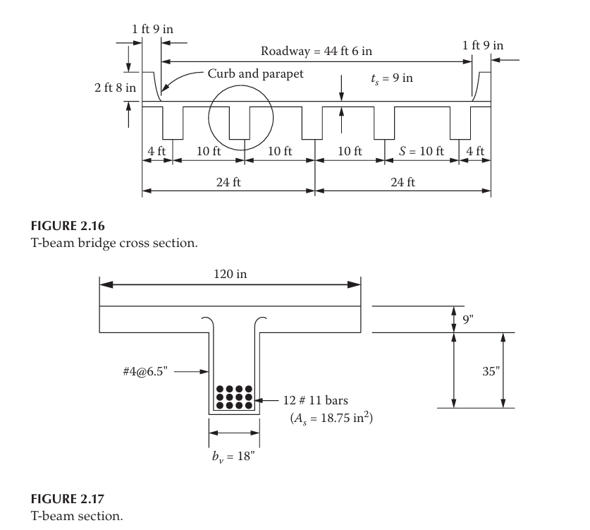
T-beam bridge cross section — five stems at 10 ft, 9-inch deck, 4-foot overhangs, 32-inch parapets — Figure 4.7T-beam cross section used throughout the Ch 4 worked example.

Step 1 — Check applicability of the empirical DF

Formula (AASHTO Table 4.6.2.2.1-1 limits)
$3.5 \le S \le 16.0\ \text{ft}, \ \ 4.5 \le t_{s} \le 12.0\ \text{in}, \ \ 20 \le L \le 240\ \text{ft}, \ \ N_{b} \ge 4$

Substitute: S = 10 ft ✓, t_s = 9 in ✓, L = 50 ft ✓, N_b = 5 ✓. Empirical DF applies. Assumed longitudinal stiffness parameter (from §3.5 procedure):K_g ≈ 250 000 in⁴.

Figure 4.8Interior tributary width (S = 10 ft) and exterior lever-rule geometry.

Step 2 — Interior girder moment DF

Formula (AASHTO 4.6.2.2.2b-1)
$DFM_{1} = 0.06 + \left(\tfrac{S}{14}\right)^{0.4} \cdot \left(\tfrac{S}{L}\right)^{0.3} \cdot \left[\tfrac{K_{g}}{12 \cdot L \cdot t_{s}^{3}}\right]^{0.1}, \quad DFM_{2+} = 0.075 + \left(\tfrac{S}{9.5}\right)^{0.6} \cdot \left(\tfrac{S}{L}\right)^{0.2} \cdot \left[\tfrac{K_{g}}{12 \cdot L \cdot t_{s}^{3}}\right]^{0.1}$
Compute the stiffness group once
$\left[\tfrac{K_{g}}{12 \cdot L \cdot t_{s}^{3}}\right]^{0.1} = \left[\tfrac{250{,}000}{12 \cdot 50 \cdot 9^{3}}\right]^{0.1} = [0.572]^{0.1} = 0.946$
Substitute — one lane
$DFM_{1} = 0.06 + (10/14)^{0.4} \cdot (10/50)^{0.3} \cdot 0.946 = 0.06 + 0.876 \cdot 0.617 \cdot 0.946 = 0.571$
Substitute — two or more lanes
$DFM_{2+} = 0.075 + (10/9.5)^{0.6} \cdot (10/50)^{0.2} \cdot 0.946 = 0.075 + 1.031 \cdot 0.725 \cdot 0.946 = 0.782$
Result
$DFM_{int} = 0.782\ \text{lanes/girder}\ \text{(governs)}$

Step 3 — Interior girder shear DF

Formula (AASHTO 4.6.2.2.3a-1)
$DFV_{1} = 0.36 + \tfrac{S}{25.0}, \quad DFV_{2+} = 0.2 + \tfrac{S}{12} - \left(\tfrac{S}{35}\right)^{2.0}$
Substitute
$DFV_{1} = 0.36 + 10/25 = 0.760$
Substitute
$DFV_{2+} = 0.2 + 10/12 - (10/35)^{2.0} = 0.2 + 0.833 - 0.082 = 0.951$
Result
$DFV_{int} = 0.951\ \text{lanes/girder}\ \text{(governs)}$

Step 4 — Exterior girder, one lane loaded (lever rule)

Formula. Assume the deck acts as a simple beam pinned at the first interior girder. Taking ΣM about that pin, and calling the two wheel lever arms a₁ and a₂:

Moment equilibrium
$R_{ext} \cdot S = \tfrac{P}{2} \cdot a_{1} + \tfrac{P}{2} \cdot a_{2} \ \Rightarrow\ g_{ext} = \tfrac{R_{ext}}{P} = \tfrac{a_{1} + a_{2}}{2S}$
Substitute
$g_{ext} = \tfrac{8.0 + 2.0}{2 \cdot 10} = 0.500$
Overhang 4 ft; exterior girder is 4 ft inboard of barrier face (d_e ≈ 2.0 ft after 2 ft barrier). Place the outer wheel 2 ft from the barrier face (§3.6.1.3.1) and the second wheel 6 ft further. Distances from the interior pin: a1 = 8.0 ft, a2 = 2.0 ft.
Apply multiple-presence (m = 1.20 for one loaded lane; lever rule does not embed m)
$DFM_{ext,\ 1\text{-}lane} = m \cdot g_{ext} = 1.20 \cdot 0.500$
Result
$DFM_{ext,\ 1\text{-}lane} = 0.600$

Figure 4.9Lever-rule free-body diagram — deck strip pinned at interior girder.

Step 5 — Exterior girder, two or more lanes loaded

Formula (AASHTO 4.6.2.2.2d-1)
$e = 0.77 + \tfrac{d_{e}}{9.1}, \quad DFM_{ext,\ 2+} = e \cdot DFM_{int,\ 2+}$
Substitute — d_e = 2.0 ft
$e = 0.77 + 2.0/9.1 = 0.990$
$DFM_{ext,\ 2+} = 0.990 \cdot 0.782 = 0.774$
Result
$DFM_{ext} = 0.774\ \text{(two-lane case, governs)}$

Step 6 — HL-93 per-lane midspan moment and end shear

Formula. Simple beam of span L with three axles P₁, P₂, P₃ placed for maximum midspan moment (Barré's theorem: the resultant and the section are equidistant from midspan):

Formula
$M_{truck} = \sum P_{i} \cdot \eta_{M,i}, \quad M_{lane} = \tfrac{w \cdot L^{2}}{8}$
Substitute — design truck (8 + 32 + 32 kip, spacings 14 ft + 14 ft)
$M_{truck} = 32 \cdot 12.5 + 32 \cdot 5.5 + 8 \cdot (-1.5) \approx 564\ \text{kip-ft/lane}$
Substitute — design tandem
$M_{tandem} = 25 \cdot (12.5 + 10.5) = 575\ \text{kip-ft/lane}\ \text{(governs)}$
Substitute — lane load
$M_{lane} = \tfrac{0.640 \cdot 50^{2}}{8} = 200\ \text{kip-ft/lane}$
Add dynamic allowance (IM = 33% on truck/tandem only; lane load excluded)
$M_{LL+IM} = (1 + IM) \cdot \max(M_{truck}, M_{tandem}) + M_{lane} = 1.33 \cdot 575 + 200 = 965\ \text{kip-ft/lane}$
End shear (truck at support, heavy axle over reaction, second axle 14 ft in, third at 28 ft)
$V_{truck} = 32 \cdot 1.0 + 32 \cdot (1 - 14/50) + 8 \cdot (1 - 28/50) = 32 + 23.0 + 3.5 = 58.5\ \text{kip/lane}$
$V_{lane} = \tfrac{w \cdot L}{2} = \tfrac{0.640 \cdot 50}{2} = 16.0\ \text{kip/lane}$
Result
$V_{LL+IM} = 1.33 \cdot 58.5 + 16.0 = 93.8\ \text{kip/lane}$

Figure 4.10HL-93 design truck placed for maximum midspan moment on a 50-ft simple span.

Step 7 — Design live-load force effects per girder

Formula — multiply per-lane envelope by the governing DF
$M_{LL+IM,\ girder} = DFM \cdot M_{LL+IM}, \quad V_{LL+IM,\ girder} = DFV \cdot V_{LL+IM}$
Substitute — moment
$M_{int} = 0.782 \cdot 965 = 755\ \text{kip-ft}, \quad M_{ext} = 0.774 \cdot 965 = 747\ \text{kip-ft}$
Substitute — shear
$V_{int} = 0.951 \cdot 93.8 = 89.2\ \text{kip}, \quad V_{ext} = (DFV_{ext} \approx 0.855) \cdot 93.8 = 80.2\ \text{kip}$

Interior girder governs both moment and shear. These per-girder values feed Strength I in Chapter 3 and the resistance design of Chapter 6.

4.6 — Software

QConBridge — HL-93 live-load analysis

QConBridge is a free, open-source Windows program developed by the Washington State Department of Transportation (WSDOT) under the Alternate Route Project. It performs live-load analysis of continuous bridge frames using the AASHTO LRFD HL-93 notional load model — the same envelope you built by hand in Step 6 — and reports Strength I, Service I/II/III, and Fatigue combinations. It is a useful check-tool: it does not size members, but it will give you the moment and shear envelopes that any hand placement of HL-93 should match.

Reference: WSDOT Bridge Engineering Software, QConBridge Overview (apps.wsdot.wa.gov). Version 1.3 (2005) — legacy but still runs on 32-bit Windows/WINE and is the standard teaching tool for LRFD live-load envelopes.

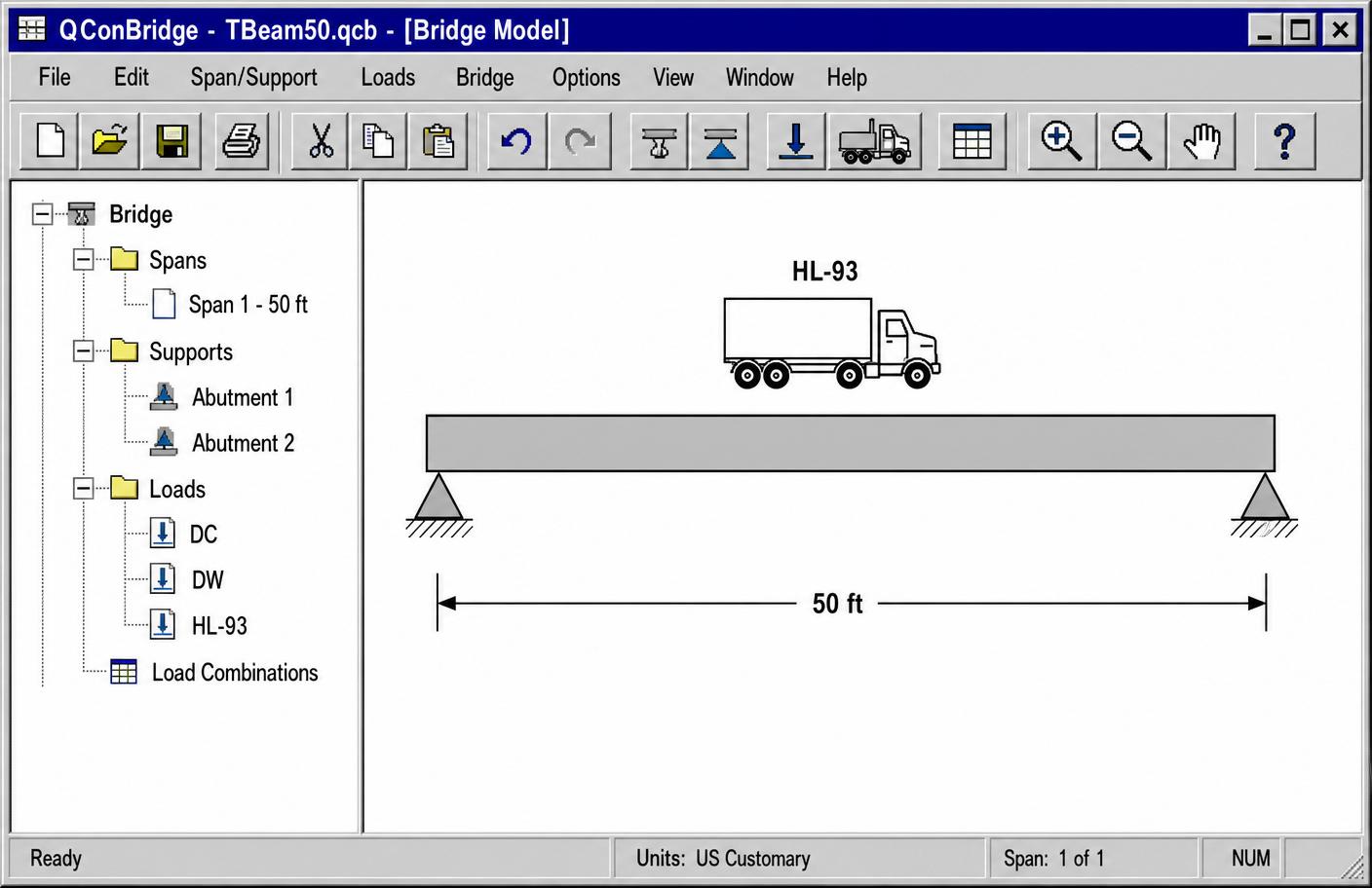
QConBridge software main window showing a simply supported 50 ft beam model with HL-93 truck — Figure 4.11QConBridge main window. Left: tree view of spans, supports, loads (DC, DW, HL-93), and load combinations. Right: bridge model canvas showing the 50-ft simple-span T-beam of §4.5.

4.6.1 Modeling procedure — one span at a time

Bridge → New. Choose US Customary units. Set number of spans (1 for our T-beam example; enter the actual number for continuous bridges) and enter each span length. For our example: 1 span, L = 50 ft.
Span/Support → Support Properties. Model both ends of the T-beam as pinned/roller abutments. For a continuous bridge, set intermediate supports as continuous (moment continuity) and leave one end free to translate longitudinally.
Span/Support → Section Properties. Enter A, I, and material E for the composite T-beam. Use the values from §3.5 / §3.7.2: for our beam, A_c, I_g, and E_c = 57 000·√f'c psi. For continuous bridges, enter separate positive-moment and negative-moment properties over the pier regions.
Loads → DC. Add uniform DC1 (girder self-weight + slab tributary) and DC2 (barriers + wearing surface if applicable) as klf on each span. From your Ch 3 calculation for the interior girder: w_DC1 ≈ 1.31 klf, w_DC2 ≈ 0.145 klf.
Loads → DW. Add the future wearing surface (0.030 ksf · tributary width) as a separate uniform load so its 1.50 load factor is applied correctly.
Loads → HL-93. Enable Design Truck, Design Tandem, and Design Lane Load. Set IM = 33% (default). For continuous bridges also enable the Dual Tandem Truck Train for the negative-moment 90% envelope (AASHTO §3.6.1.3.1).
Bridge → Distribution Factors. Enter the DFs you hand-computed in Steps 2–5. Enter DFM_int = 0.782, DFM_ext = 0.774, DFV_int = 0.951, DFV_ext = 0.855. QConBridge will multiply the per-lane envelopes by these DFs.
Analyze → Run. The solver assembles the influence lines, positions HL-93 for each envelope station, and combines with DC / DW using AASHTO §3.4.1 factors.
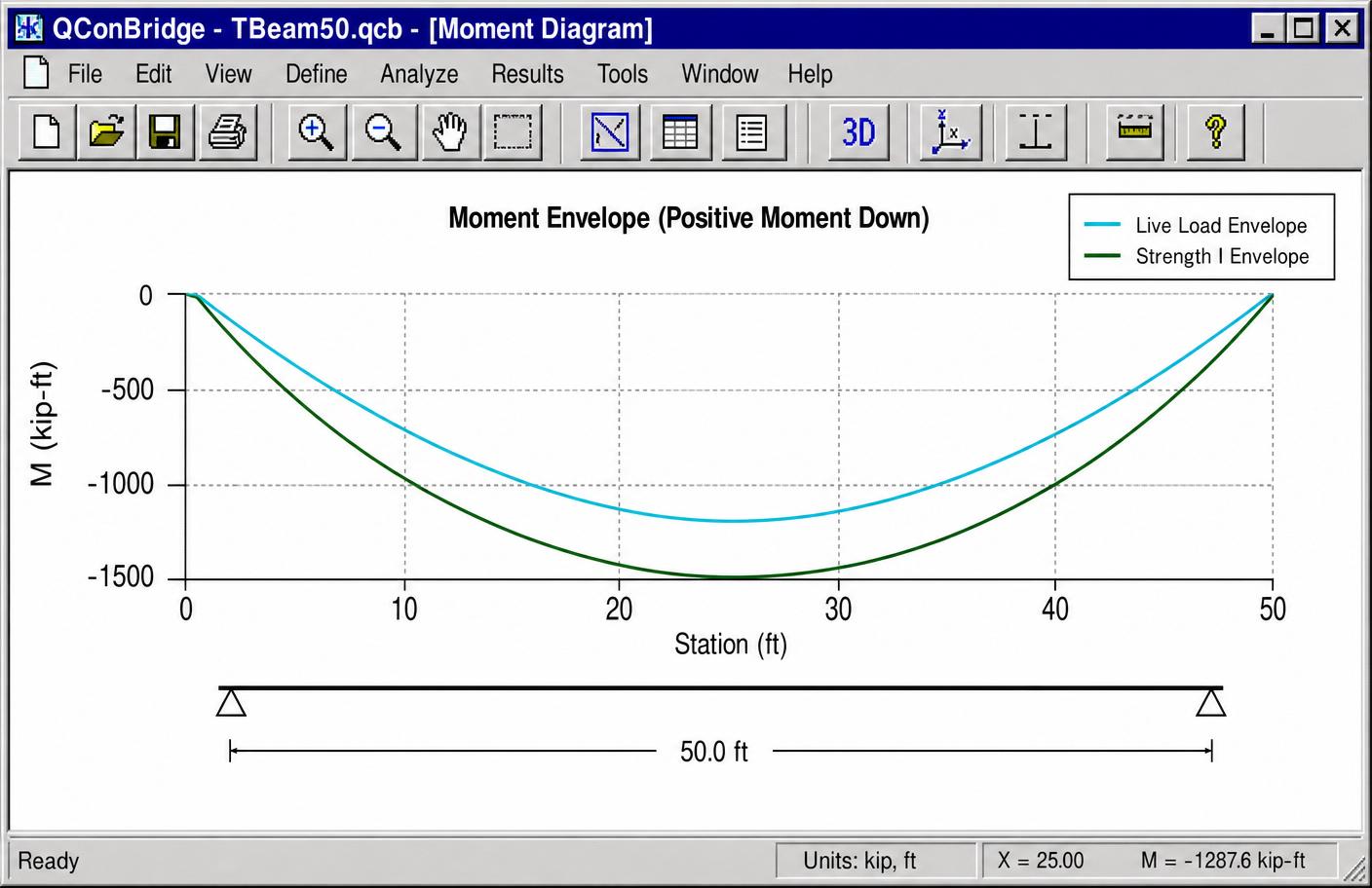
Results → Moment Diagram / Shear Diagram / Reactions. Choose the load combination (Live Load Envelope, Strength I, Service I, Fatigue). Right-click the plot to export tabular results.

QConBridge moment diagram window showing Live Load Envelope and Strength I Envelope for a 50 ft span — Figure 4.12QConBridge output window — moment envelope for the 50-ft T-beam. The Strength I curve peaks at −1288 kip-ft at midspan; compare with the hand result of Step 6 (girder-level Strength I ≈ 1250 kip-ft for the interior beam once DC/DW are added).

Hand-check every QConBridge run

Sum of reactions under DC1 alone equals w_DC1·L (statics — exact).
Midspan Live-Load Envelope moment matches your hand HL-93 positioning within 2%.
Strength I moment ≈ 1.25·M_DC1 + 1.50·M_DW + 1.75·M_LL+IM.
End shear from QConBridge equals w·L/2 (dead) plus your hand HL-93 end shear.

A discrepancy larger than 5% means either the input (DF, section, load) is wrong or your hand check is wrong. Reconcile before proceeding to design.

Alternatives

Same workflow, different tools: MDX (BridgeSoft), LEAP CONSPAN, PGSuper (also WSDOT, for prestressed girders), and full-featured FE packages CSiBridge, midas Civil, LARSA 4D. The AASHTO §4.6.3 rules for refined analysis apply to all of them.

4.7 — Design challenge

Analysis package for the T-beam bridge

This challenge picks up the analysis half of the Chapter-3 T-beam problem — the pieces that properly belong to analysis rather than to loads. Chapter 3 stops at the raw per-lane HL-93 envelopes and permanent load intensities. Use those numbers as inputs.

T-beam bridge cross section for the design challenge — Fig. 4.CH-1Same bridge as Ch 3 challenge: 44 ft 6 in roadway, 5 stems at 10 ft, 4-ft overhangs, ts = 9 in, 18 in x 35 in stems, 32-in parapets, L = 50 ft, skew = 0, f'c = 4.5 ksi, DW = 0.030 ksf.

Deliverables — for BOTH an interior and an exterior girder

Live-load distribution factors (AASHTO §4.6.2.2, cross-section type (e)): compute DFM and DFV for one-lane and two-or-more-lanes loaded, and pick the governing value. Include the lever-rule calculation for the exterior girder and the two-lane e-factor. Skew = 0°, so the skew corrections drop out — state that explicitly.
Per-lane HL-93 force effects for L = 50 ft: maximum midspan moment (envelope of design truck vs. design tandem, each with IM = 33%, plus the 0.640 klf lane load) and maximum end shear. Show the axle-placement sketch and the influence-line ordinates you used.
Design live-load M and V per girder: multiply per-lane envelopes by the governing DFs. Report M_LL+IM and V_LL+IM for interior and exterior girders.
Strength I check at midspan: assemble γ·Q for DC1, DC2, DW, and LL+IM using the DC1, DC2, DW you computed in the Ch 3 challenge. Compare to the Chapter-6 resistance target (report only the demand — no resistance yet).
QConBridge run: build the model per §4.6.1, print the moment- and shear-envelope plots, and tabulate a side-by-side comparison with your hand values. Explain any discrepancy > 5%.
Validation note: show at least three of the check items from the "hand-check every QConBridge run" callout above.

What to hand in

A single PDF containing: (a) DF calculations with formula → substitution → result for each line, (b) HL-93 axle-placement sketch and per-lane force-effect calculations, (c) per-girder M_LL+IM and V_LL+IM summary table, (d) QConBridge screenshots of the model and the two envelope plots, (e) hand-vs-software comparison table with % differences. Upload below.

Submit your design challenge

Chapter 4 challenge — T-beam bridge analysis: DFs, live-load M & V, QConBridge run

You must be signed in to upload a submission.

4.8 — Common mistakes

What to avoid

Applying two-lane DFs to a bridge that will legally carry only one loaded lane.
Forgetting the skew correction on shear DF for skewed bridges (§4.6.2.2.3c).
Using approximate distribution outside its applicability envelope (spacing, skew, span, N_b).
Double-counting the multiple-presence factor m on empirical DFs.
Failing to enforce cross-frame compatibility in a grillage (releasing torsional continuity where it belongs).
Trusting FE / QConBridge output without a hand-check envelope — statics is not optional.
Modeling a curved-girder bridge as a straight beam line — the torsional warping moments are lost.
Neglecting to update the stiffness matrix for staged construction (non-composite dead load on the bare steel, composite dead load on the composite section).

Chapter summary

Key takeaways

Every load flows: wheel → deck → girder → bearing → pier → foundation → soil. Every link introduces a modeling assumption.
Influence lines give the position that maximizes a response; the Müller-Breslau principle constructs them by inspection.
AASHTO empirical DFs collapse the two-way slab-girder problem into a one-dimensional design per girder — inside their applicability range.
The lever rule and rigid-body method handle exterior girders and cases outside empirical bounds.
Skewed bridges need the moment reduction (c₁) and the shear amplification factors from §4.6.2.2.
QConBridge (or an equivalent) automates the HL-93 envelope but is only trustworthy after a hand check on reactions, midspan moment, and Strength I.
Refined analysis (grillage, shell FE) is required for curved, deeply skewed, and non-standard bridges — and must be validated by statics.

Section 2

Fully Worked Examples

Complete AASHTO LRFD solutions with knowns, assumptions, step calculations, verification, and design commentary. Difficulty rises from basic to consulting-grade.

Worked Example 1

Distribution factor for interior girder (moment, one design lane)

Basic

Problem

Compute DF_m,int (one lane).

Step-by-Step

DF = 0.06 + (S/14)^{0.4} \cdot (S/L)^{0.3} \cdot (K_{g}/(12Lt_{s}^{3}))^{0.1}

= 0.06 + (8/14)^{0.4}\cdot (8/90)^{0.3}\cdot (1.2)^{0.1} = 0.06 + 0.799\cdot 0.481\cdot 1.018

Result

DF \approx 0.06 + 0.391 = 0.451

Design Verification

Cross-check: at S=8 ft, DF one-lane is typically 0.42–0.48 for I-girders. ✓

Discussion

Do NOT include multiple-presence factor m — Table 4.6.2.2.2b-1 formulas already include it.

Worked Example 2

Two-or-more-lanes distribution factor and controlling design

Intermediate

Problem

Compute DF_m,int (two or more) and select governing DF.

Step-by-Step

DF = 0.075 + (S/9.5)^{0.6}\cdot (S/L)^{0.2}\cdot (K_{g}/(12Lt_{s}^{3}))^{0.1}

= 0.075 + (8/9.5)^{0.6}\cdot (8/90)^{0.2}\cdot (1.2)^{0.1} = 0.075 + 0.906\cdot 0.615\cdot 1.018

Result

DF \approx 0.075 + 0.567 = 0.642

Design Verification

Two-lane usually controls for interior girders at S = 7–10 ft with normal spans. ✓

Discussion

For exterior girders, add lever-rule and rigid-body-rotation checks per §4.6.2.2.2d — they can control.

Worked Example 3

Live-load moment at midspan from HL-93 + IM

Intermediate

Problem

Compute M_LL+IM per lane, then per girder using DF = 0.642.

Step-by-Step

M_{LL+IM} = M_{LT}\cdot (1+IM) + M_{LN} = 1524\cdot 1.33 + 405

Result

2432 k\cdot ft/lane

M_{g} = DF\cdot M_{LL+IM} = 0.642\cdot 2432

Result

M_{g} = 1561 k\cdot ft

Design Verification

Truck governs positive moment for L up to ~120 ft; tandem+lane may govern shorter spans and check both. ✓

Discussion

IM applies to truck axles only, never to lane load. A common student mistake is applying (1+IM) to the full envelope.

Section 3

Guided Practice

Complete the missing steps. Use Hints for AASHTO article pointers and setup logic before revealing the full step. Submit at the end to send your work to your instructor.

Guided Problem 1

Influence line for a two-span continuous beam

A two-span continuous beam has equal spans $L = 100\ \text{ft}$ and constant $EI$ . Determine key influence-line ordinates for the reaction at the interior support and midspan-1 moment using three-moment or Müller-Breslau reasoning.

Step 1

Ordinate of $R_{B}$ (interior reaction) when the unit load sits at midspan of span 1 (dimensionless).

Answer

Step 2

Ordinate of the interior reaction when the unit load sits directly above pier B.

Answer

Step 3

Ordinate of midspan-1 moment (k-ft per kip) when the load sits at midspan-1.

Answer

Step 4

Maximum positive moment envelope at midspan-1 from AASHTO HL-93 truck (32k axles at 14 ft), placing axles to maximize the influence area. Approximate (k-ft).

Answer

Guided Problem 2

Live-load distribution factor for an interior steel I-girder

Composite steel I-girder, $S = 9\ \text{ft}$ , span $L = 120\ \text{ft}$ , deck $t_{s} = 8\ \text{in}$ , $K_{g} = 3.2 \times 10^{6}\ \text{in}^{4}$ , two design lanes loaded.

Step 1

$\left(\dfrac{K_{g}}{12 \cdot L \cdot t_{s}^{3}}\right)^{0.1}$ exponent term (dimensionless).

Answer

Step 2

$(S/9.5)^{0.6}$ .

Answer

Step 3

$(S/L)^{0.2}$ .

Answer

Step 4

Two-lane interior moment $DF = 0.075 + (S/9.5)^{0.6} \cdot (S/L)^{0.2} \cdot \left(\dfrac{K_{g}}{12Lt_{s}^{3}}\right)^{0.1}$ .

Answer

Guided Problem 3

Grillage vs strip method — same deck, two answers

A 40-ft-wide, 4-girder deck with 8-in slab, $S = 9\ \text{ft}$ . Compare deck-strip transverse moment (AASHTO §4.6.2.1) to a hand-grillage transverse moment.

Step 1

Effective strip width for positive moment (in). $E = 26 + 6.6 \cdot S(\text{ft})$ .

Answer

Step 2

Wheel load per strip (kip). Use 16 kip design wheel.

Answer

Step 3

Transverse positive moment $M = P \cdot S/4$ (k-ft/ft) for 1-ft strip with simple-span idealization.

Answer

Step 4

AASHTO Table A4-1 tabulated $M_{LL+IM}$ for $S = 9\ \text{ft}$ (k-ft/ft).

Answer

Guided Problem 4

Modal analysis: fundamental frequency estimate

Simply supported PS concrete girder bridge, span $L = 120\ \text{ft}$ , $EI = 8.5 \times 10^{10}\ \text{lb} \cdot \text{in}^{2}$ , self-weight $w = 3.2\ \text{klf}$ including deck.

Step 1

Mass per unit length $\mu$ (kip·s²/ft²). Use $g = 32.2\ \text{ft/s}^{2}$ .

Answer

Step 2

Convert $EI$ to kip·ft². Divide by $144 \cdot 1000$ .

Answer

Step 3

$f_{1} = \dfrac{\pi}{2L^{2}} \sqrt{\dfrac{EI}{\mu}}$ in Hz.

Answer

Step 4

Does the bridge fall into the pedestrian-uncomfortable range ( $1.6\text{–}2.4\ \text{Hz}$ )?

Answer

Section 4

Independent Practice

Every problem randomizes its inputs. Work each step, submit for immediate feedback, request new values to practice again.

Practice 1

Simple-span moment from uniform load

w = 3.3000000000000003 klf

Span

L = 175 ft

Step 1w·L²/8.

Answer (k-ft)

Randomized inputs, symbolic grading (±2%).

Practice 2

Concentrated axle moment (simply supported)

Axle

P = 12 kip

Span

L = 110 ft

Step 1P·L/4.

Answer (k-ft)

Randomized inputs, symbolic grading (±2%).

Practice 3

Two-equal-span continuous, uniform load — interior reaction

w = 1.6 klf

Span

L = 70 ft

Step 1R_B = 1.25·w·L.

Answer (kip)

Randomized inputs, symbolic grading (±2%).

Practice 4

Fixed-end moment (uniform)

w = 3.8000000000000003 klf

Span

L = 90 ft

Step 1w·L²/12.

Answer (k-ft)

Randomized inputs, symbolic grading (±2%).

Practice 5

Live-load DF (two-lane interior moment, quick form)

S = 7 ft

Span

L = 100 ft

Step 10.075 + (S/9.5)^0.6·(S/L)^0.2 (Kg-term ≈ 1).

Answer (-)

Randomized inputs, symbolic grading (±2%).

Practice 6

Deck strip width E for positive moment

S = 7.5 ft

Step 1E = 26 + 6.6·S (in).

Answer (in)

Randomized inputs, symbolic grading (±2%).

Practice 7

Impact factor on truck moment

M_truck

M = 925 k-ft

Step 1×1.33.

Answer (k-ft)

Randomized inputs, symbolic grading (±2%).

Practice 8

First natural frequency of a simple beam

EI (kip·ft²)

EI = 500000 kip·ft^2

μ (kip·s²/ft²)

mu = 0.135 -

Span

L = 190 ft

Step 1f_1 = (π/(2L²))·√(EI/μ).

Answer (Hz)

Randomized inputs, symbolic grading (±2%).

Practice 9

Multi-lane factor m

Loaded lanes

n = 2 -

Step 1AASHTO Table 3.6.1.1.2-1 multi-presence factor.

Answer (-)

Randomized inputs, symbolic grading (±2%).

Practice 10

Deflection of simple beam (uniform)

w = 2.8000000000000003 klf

Span

L = 140 ft

EI (kip·ft²)

EI = 600000 -

Step 15·w·L⁴/(384·EI) (ft).

Answer (ft)

Step 2×12.

Answer (in)

Randomized inputs, symbolic grading (±2%).

Practice 11

Truck reaction, straddle two spans

Axle

P = 26 kip

Span

L = 95 ft

Distance from support

a = 15 ft

Step 1R = P·(L−a)/L.

Answer (kip)

Randomized inputs, symbolic grading (±2%).

Practice 12

Cantilever tip deflection under point load

P = 22 kip

Cantilever

L = 30 ft

EI (kip·ft²)

EI = 750000 -

Step 112·P·L³/(3·EI).

Answer (in)

Randomized inputs, symbolic grading (±2%).